Tutorial: Build an ETL pipeline using change data capture
You create and deploy an ETL (extract, transform, and load) pipeline with change data capture (CDC) using Lakeflow pipelines for data orchestration and Auto Loader. An ETL pipeline implements the steps to read data from source systems, transform that data based on requirements, such as data quality checks and record de-duplication, and write the data to a target system, such as a data warehouse or a data lake.
In this tutorial, you'll use data from a customers table in a MySQL database to:
- Extract the changes from a transactional database using Debezium or another tool and save them to cloud object storage (S3, ADLS, or GCS). In this tutorial, you skip setting up an external CDC system and instead generate fake data to simplify the tutorial.
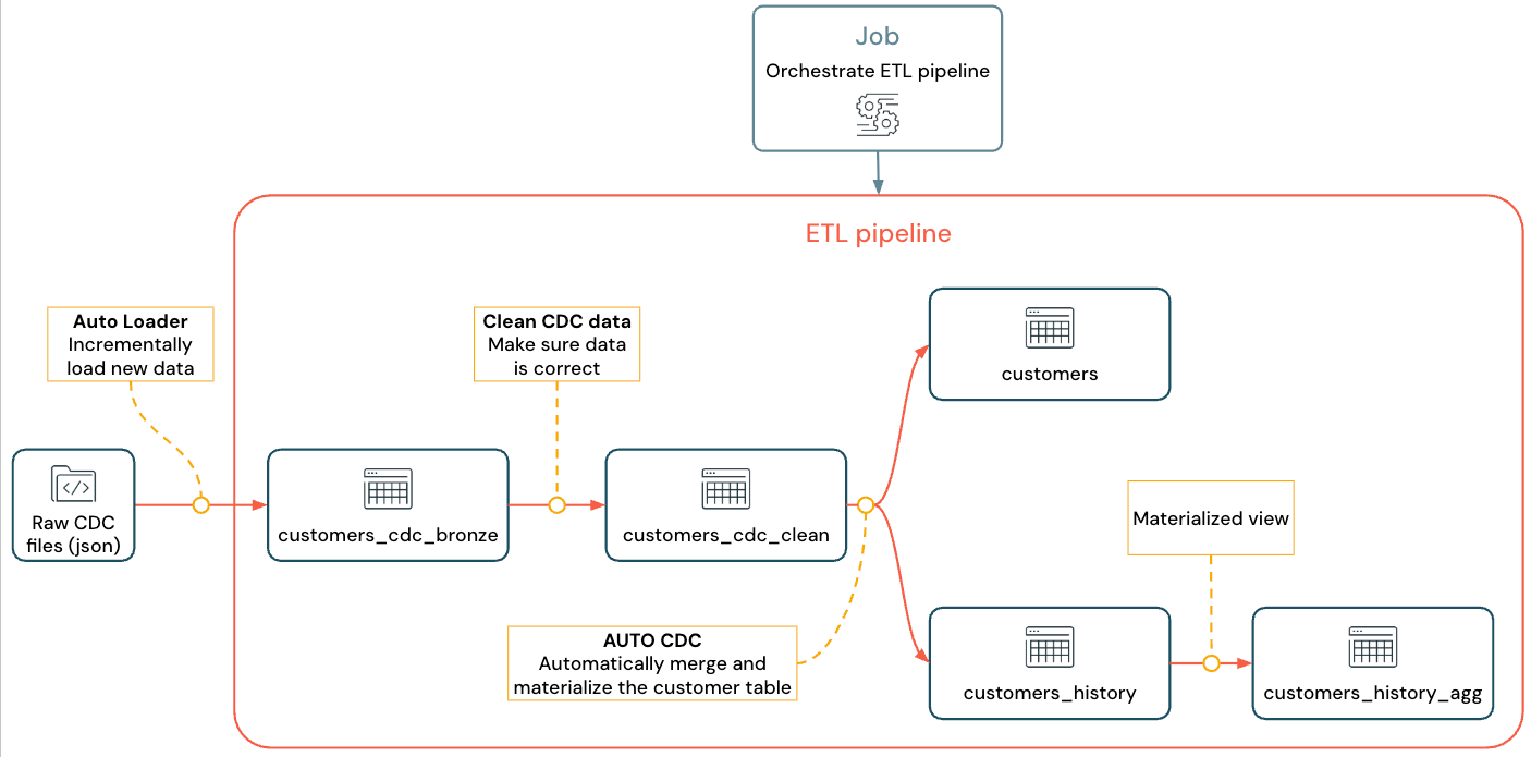
- Use Auto Loader to incrementally load the messages from cloud object storage, and store the raw messages in the
customers_cdctable. Auto Loader infers the schema and handles schema evolution. - Create the
customers_cdc_cleantable to check data quality using expectations. For example, theidshould never benullbecause it's used to run upsert operations. - Perform
AUTO CDC ... INTOon the cleaned CDC data to upsert changes into the finalcustomerstable. - Show how a pipeline can create a type 2 slowly changing dimension (SCD2) table to track all changes.
The goal is to ingest the raw data in near real time and build a table for your analyst team while ensuring data quality.
The tutorial uses the medallion Lakehouse architecture, where it ingests raw data through the bronze layer, cleans and validates data with the silver layer, and applies dimensional modeling and aggregation using the gold layer. See What is the medallion lakehouse architecture? for more information.
The implemented flow looks like this:
For more information about pipeline, Auto Loader, and CDC see Spark Declarative Pipelines, What is Auto Loader?, and Change data capture and snapshots
Requirements
To complete this tutorial, you must meet the following requirements:
- Unity Catalog is enabled for your workspace.
- Serverless compute is available in your workspace (enabled by default in workspaces with Unity Catalog). Serverless Lakeflow pipelines are not available in all workspace regions. See Features with limited regional availability for available regions. If serverless compute is not available, the steps should work with the default compute for your workspace.
- Permission to create a compute resource or access to a compute resource.
- Permissions to create a new schema in a catalog. The required permissions are
USE CATALOGandCREATE SCHEMA. - Permissions to create a new volume in an existing schema. The required permissions are
USE SCHEMAandCREATE VOLUME. - For the full set of privileges required to create, run, refresh, and view pipelines and their output, see Manage identities, permissions, and privileges for pipelines.
Change data capture in an ETL pipeline
Change data capture (CDC) is the process that captures changes in records made to a transactional database (for example, MySQL or PostgreSQL) or a data warehouse. CDC captures operations like data deletes, appends, and updates, typically as a stream to re-materialize tables in external systems. CDC enables incremental loading while eliminating the need for bulk-load updates.
To simplify this tutorial, skip setting up an external CDC system. Assume it's running and saving CDC data as JSON files in cloud object storage (S3, ADLS, or GCS). This tutorial uses the Faker library to generate the data used in the tutorial.
Capturing CDC
A variety of CDC tools are available. One of the leading open source solutions is Debezium, but other implementations that simplify data sources exist, such as Fivetran, Qlik Replicate, StreamSets, Talend, Oracle GoldenGate, and AWS DMS.
In this tutorial, you use CDC data from an external system like Debezium or DMS. Debezium captures every changed row. It typically sends the history of data changes to Kafka topics or saves them as files.
You must ingest the CDC information from the customers table (JSON format), check that it is correct, and then materialize the customers table in the Lakehouse.
CDC input from Debezium
For each change, you receive a JSON message containing all the fields of the row being updated (id, firstname, lastname, email, address). The message also includes additional metadata:
operation: An operation code, typically (DELETE,APPEND,UPDATE).operation_date: The date and timestamp for the record for each operation action.
Tools like Debezium can produce more advanced output, such as the row value before the change, but this tutorial omits them for simplicity.
Step 1: Create a pipeline
Create a new ETL pipeline to query your CDC data source and generate tables in your workspace.
-
In your workspace, click
 New in the sidebar, then select ETL Pipeline. This opens the pipeline editor with a default pipeline name like
 New Pipeline <date> <time>. -
Select the name and enter a descriptive name, such as
Pipelines with CDC tutorial. -
To the right of the name, click the catalog and schema to choose defaults for which you have write permissions.
This catalog and schema are used by default, if you do not specify a catalog or schema in your code. Your code can write to any catalog or schema by specifying the full path. This tutorial uses the defaults that you specify here.
-
(Optional) In the
my_transformationsource file created for you, select Python or SQL from the language drop-down list to set the language for the file. -
Click
 Use sample code.
The Lakeflow Pipelines Editor opens with sample files in your pipeline. You will add your own transformation files in later steps. Next, set up the sample data to import in the tutorial.
Step 2: Create the sample data to import in this tutorial
This step is not needed if you are importing your own data from an existing source. For this tutorial, generate fake data as an example for the tutorial. Create a notebook to run the Python data generation script. This code only needs to be run once to generate the sample data, so create it within the pipeline's explorations folder, which is not run as part of a pipeline update.
This code uses Faker to generate the sample CDC data. Faker is available to install automatically, so the tutorial uses %pip install faker. You can also set a dependency on faker for the notebook. See Add dependencies to the notebook.
-
From within the Lakeflow Pipelines Editor, in the asset browser sidebar to the left of the editor, click
Add, then choose Exploration. -
Give it a Name, such as
Setup data, select Python. You can leave the default destination folder, which is a newexplorationsfolder. -
Click Create. This creates a notebook in the new folder.
-
Enter the following code in the first cell. You must change the definition of
<my_catalog>and<my_schema>to match the default catalog and schema that you selected in the previous procedure:Python%pip install faker
# Update these to match the catalog and schema
# that you used for the pipeline in step 1.
catalog = "<my_catalog>"
schema = dbName = db = "<my_schema>"
spark.sql(f'USE CATALOG `{catalog}`')
spark.sql(f'USE SCHEMA `{schema}`')
spark.sql(f'CREATE VOLUME IF NOT EXISTS `{catalog}`.`{db}`.`raw_data`')
volume_folder = f"/Volumes/{catalog}/{db}/raw_data"
try:
dbutils.fs.ls(volume_folder+"/customers")
except:
print(f"folder doesn't exist, generating the data under {volume_folder}...")
from pyspark.sql import functions as F
from faker import Faker
from collections import OrderedDict
import uuid
fake = Faker()
import random
fake_firstname = F.udf(fake.first_name)
fake_lastname = F.udf(fake.last_name)
fake_email = F.udf(fake.ascii_company_email)
fake_date = F.udf(lambda:fake.date_time_this_month().strftime("%m-%d-%Y %H:%M:%S"))
fake_address = F.udf(fake.address)
operations = OrderedDict([("APPEND", 0.5),("DELETE", 0.1),("UPDATE", 0.3),(None, 0.01)])
fake_operation = F.udf(lambda:fake.random_elements(elements=operations, length=1)[0])
fake_id = F.udf(lambda: str(uuid.uuid4()) if random.uniform(0, 1) < 0.98 else None)
df = spark.range(0, 100000).repartition(100)
df = df.withColumn("id", fake_id())
df = df.withColumn("firstname", fake_firstname())
df = df.withColumn("lastname", fake_lastname())
df = df.withColumn("email", fake_email())
df = df.withColumn("address", fake_address())
df = df.withColumn("operation", fake_operation())
df_customers = df.withColumn("operation_date", fake_date())
df_customers.repartition(100).write.format("json").mode("overwrite").save(volume_folder+"/customers") -
To generate the dataset used in the tutorial, type Shift + Enter to run the code:
-
Optional. To preview the data used in this tutorial, enter the following code in the next cell and run the code. Update the catalog and schema to match the path from the previous code.
Python# Update these to match the catalog and schema
# that you used for the pipeline in step 1.
catalog = "<my_catalog>"
schema = "<my_schema>"
display(spark.read.json(f"/Volumes/{catalog}/{schema}/raw_data/customers"))
This generates a large data set (with fake CDC data) that you can use in the rest of the tutorial. In the next step, ingest the data using Auto Loader.
Step 3: Incrementally ingest data with Auto Loader
The next step is to ingest the raw data from the (faked) cloud storage into a bronze layer.
This can be challenging for multiple reasons, as you must:
- Operate at scale, potentially ingesting millions of small files.
- Infer schema and JSON type.
- Handle bad records with incorrect JSON schema.
- Take care of schema evolution (for example, a new column in the customer table).
Auto Loader simplifies this ingestion, including schema inference and schema evolution, while scaling to millions of incoming files. Auto Loader is available in Python using cloudFiles and in SQL using the SELECT * FROM STREAM read_files(...) and can be used with a variety of formats (JSON, CSV, Apache Avro, etc.):
Defining the table as a streaming table guarantees that you only consume new incoming data. If you do not define it as a streaming table, it scans and ingests all the available data. See Streaming tables for more information.
-
To ingest the incoming CDC data using Auto Loader, copy and paste the following code into the code file that was created with your pipeline (called
my_transformation.pyormy_transformation.sql). You can use Python or SQL, based on the language you chose when creating the pipeline. Be sure to replace the<catalog>and<schema>with the ones that you set up for the default for the pipeline.- Python
- SQL
Pythonfrom pyspark import pipelines as dp
from pyspark.sql.functions import *
# Replace with the catalog and schema name that
# you are using:
path = "/Volumes/<catalog>/<schema>/raw_data/customers"
# Create the target bronze table
dp.create_streaming_table("customers_cdc_bronze", comment="New customer data incrementally ingested from cloud object storage landing zone")
# Create an Append Flow to ingest the raw data into the bronze table
@dp.append_flow(
target = "customers_cdc_bronze",
name = "customers_bronze_ingest_flow"
)
def customers_bronze_ingest_flow():
return (
spark.readStream
.format("cloudFiles")
.option("cloudFiles.format", "json")
.option("cloudFiles.inferColumnTypes", "true")
.load(f"{path}")
)SQLCREATE OR REFRESH STREAMING TABLE customers_cdc_bronze
COMMENT "New customer data incrementally ingested from cloud object storage landing zone";
CREATE FLOW customers_bronze_ingest_flow AS
INSERT INTO customers_cdc_bronze BY NAME
SELECT *
FROM STREAM read_files(
-- replace with the catalog/schema you are using:
"/Volumes/<catalog>/<schema>/raw_data/customers",
format => "json",
inferColumnTypes => "true"
) -
Click
 Run file or Run pipeline to start an update for the connected pipeline. With only one source file in your pipeline, these are functionally equivalent.
When the update completes, the editor is updated with information about your pipeline.
- The pipeline graph, also called the directed acyclic graph (DAG), in the sidebar to the right of your code, shows a single table,
customers_cdc_bronze. - A summary of the update is shown at the top of the pipeline asset browser.
- Details of the table that was generated are shown in the bottom pane, and you can browse data from the table by selecting it.
This is the raw bronze layer data imported from cloud storage. In the next step, clean the data to create a silver layer table.
Step 4: Cleanup and expectations to track data quality
After the bronze layer is defined, create the silver layer by adding expectations to control data quality. Check the following conditions:
- ID must never be
null. - The CDC operation type must be valid.
- JSON must be read correctly by Auto Loader.
Rows that don't meet these conditions are dropped.
See Manage data quality with pipeline expectations for more information.
-
From the pipeline asset browser sidebar, click
Add, then Transformation. -
Enter a Name (for example,
customers_silver) and choose a language (Python or SQL) for the source code file. The.pyor.sqlextension is appended based on your language choice. You can mix and match languages within a pipeline, so you can choose either one for this step. -
To create a silver layer with a cleansed table and impose constraints, copy and paste the following code into the new file (choose Python or SQL based on the language of the file).
- Python
- SQL
Pythonfrom pyspark import pipelines as dp
from pyspark.sql.functions import *
dp.create_streaming_table(
name = "customers_cdc_clean",
expect_all_or_drop = {"no_rescued_data": "_rescued_data IS NULL","valid_id": "id IS NOT NULL","valid_operation": "operation IN ('APPEND', 'DELETE', 'UPDATE')"}
)
@dp.append_flow(
target = "customers_cdc_clean",
name = "customers_cdc_clean_flow"
)
def customers_cdc_clean_flow():
return (
spark.readStream.table("customers_cdc_bronze")
.select("address", "email", "id", "firstname", "lastname", "operation", "operation_date", "_rescued_data")
)SQLCREATE OR REFRESH STREAMING TABLE customers_cdc_clean (
CONSTRAINT no_rescued_data EXPECT (_rescued_data IS NULL) ON VIOLATION DROP ROW,
CONSTRAINT valid_id EXPECT (id IS NOT NULL) ON VIOLATION DROP ROW,
CONSTRAINT valid_operation EXPECT (operation IN ('APPEND', 'DELETE', 'UPDATE')) ON VIOLATION DROP ROW
)
COMMENT "New customer data incrementally ingested from cloud object storage landing zone";
CREATE FLOW customers_cdc_clean_flow AS
INSERT INTO customers_cdc_clean BY NAME
SELECT * FROM STREAM customers_cdc_bronze; -
Click
Run file or Run pipeline to start an update for the connected pipeline.Because there are now two source files, these do not do the same thing, but in this case, the output is the same.
- Run pipeline runs your entire pipeline, including the code from step 3. If your input data were being updated, this would pull in any changes from that source to your bronze layer. This does not run the code from the data setup step, because that is in the explorations folder, and not part of the source for your pipeline.
- Run file runs only the current source file. In this case, without your input data being updated, this generates the silver data from the cached bronze table. It would be useful to run just this file for faster iteration when creating or editing your pipeline code.
When the update completes, you can see that the pipeline graph now shows two tables (with the silver layer depending on the bronze layer), and the bottom panel shows details for both tables. The top of the pipeline asset browser now shows multiple runs' times, but only details for the most recent run.
Next, create your final gold layer version of the customers table.
Step 5: Materialize the customers table with an AUTO CDC flow
Up to this point, the tables have just passed the CDC data along in each step. Now, create the customers table to both contain the most up-to-date view and to be a replica of the original table, not the list of CDC operations that created it.
This is nontrivial to implement manually. You must consider things like data deduplication to keep the most recent row.
However, pipelines solve these challenges with the AUTO CDC operation.
-
From the pipeline asset browser sidebar, click
Add and Transformation. -
Enter a Name and choose a language (Python or SQL) for the new source code file. You can again choose either language for this step, but use the correct code, below.
-
To process the CDC data using
AUTO CDC, copy and paste the following code into the new file.- Python
- SQL
Pythonfrom pyspark import pipelines as dp
from pyspark.sql.functions import *
dp.create_streaming_table(name="customers", comment="Clean, materialized customers")
dp.create_auto_cdc_flow(
target="customers", # The customer table being materialized
source="customers_cdc_clean", # the incoming CDC
keys=["id"], # what we'll be using to match the rows to upsert
sequence_by=col("operation_date"), # de-duplicate by operation date, getting the most recent value
ignore_null_updates=False,
apply_as_deletes=expr("operation = 'DELETE'"), # DELETE condition
except_column_list=["operation", "operation_date", "_rescued_data"],
)SQLCREATE OR REFRESH STREAMING TABLE customers;
CREATE FLOW customers_cdc_flow
AS AUTO CDC INTO customers
FROM stream(customers_cdc_clean)
KEYS (id)
APPLY AS DELETE WHEN
operation = "DELETE"
SEQUENCE BY operation_date
COLUMNS * EXCEPT (operation, operation_date, _rescued_data)
STORED AS SCD TYPE 1; -
Click
Run file to start an update for the connected pipeline.
When the update is complete, you can see that your pipeline graph shows 3 tables, progressing from bronze to silver to gold.
Step 6: Track update history with slowly changing dimension type 2 (SCD2)
It's often required to create a table tracking all the changes resulting from APPEND, UPDATE, and DELETE:
- History: You want to keep a history of all the changes to your table.
- Traceability: You want to see which operation occurred.
SCD2 with Lakeflow pipelines
Delta supports change data flow (CDF), and table_change can query table modifications in SQL and Python. However, CDF's main use case is to capture changes in a pipeline, not to create a full view of table changes from the beginning.
Things get especially complex to implement if you have out-of-order events. If you must sequence your changes by a timestamp and receive a modification that happened in the past, you must append a new entry in your SCD table and update the previous entries.
Lakeflow pipelines remove this complexity. You can create a separate table that contains all modifications from the beginning of time, which the pipeline maintains automatically. This table supports data layout optimizations such as liquid clustering and handles out-of-order records automatically based on _sequence_by. See Use liquid clustering for tables.
To create an SCD2 table, use the option STORED AS SCD TYPE 2 in SQL or stored_as_scd_type="2" in Python.
You can also limit which columns the feature tracks using the option: TRACK HISTORY ON {columnList | EXCEPT(exceptColumnList)}
-
From the pipeline asset browser sidebar, click
Add and Transformation. -
Enter a Name and choose a language (Python or SQL) for the new source code file.
-
Copy and paste the following code into the new file.
- Python
- SQL
Pythonfrom pyspark import pipelines as dp
from pyspark.sql.functions import *
# create the table
dp.create_streaming_table(
name="customers_history", comment="Slowly Changing Dimension Type 2 for customers"
)
# store all changes as SCD2
dp.create_auto_cdc_flow(
target="customers_history",
source="customers_cdc_clean",
keys=["id"],
sequence_by=col("operation_date"),
ignore_null_updates=False,
apply_as_deletes=expr("operation = 'DELETE'"),
except_column_list=["operation", "operation_date", "_rescued_data"],
stored_as_scd_type="2",
) # Enable SCD2 and store individual updatesSQLCREATE OR REFRESH STREAMING TABLE customers_history;
CREATE FLOW customers_history_cdc
AS AUTO CDC INTO
customers_history
FROM stream(customers_cdc_clean)
KEYS (id)
APPLY AS DELETE WHEN
operation = "DELETE"
SEQUENCE BY operation_date
COLUMNS * EXCEPT (operation, operation_date, _rescued_data)
STORED AS SCD TYPE 2; -
Click
Run file to start an update for the connected pipeline.
When the update is complete, the pipeline graph includes the new customers_history table, also dependent on the silver layer table, and the bottom panel shows the details for all 4 tables.
Step 7: Create a materialized view that tracks who has changed their information the most
The table customers_history contains all historical changes a user has made to their information. Create a simple materialized view in the gold layer that keeps track of who has changed their information the most. This could be used for fraud detection analysis or user recommendations in a real-world scenario. Additionally, applying changes with SCD2 has already removed duplicates, so you can directly count the rows per user ID.
-
From the pipeline asset browser sidebar, click
Add and Transformation. -
Enter a Name and choose a language (Python or SQL) for the new source code file.
-
Copy and paste the following code into the new source file.
- Python
- SQL
Pythonfrom pyspark import pipelines as dp
from pyspark.sql.functions import *
@dp.table(
name = "customers_history_agg",
comment = "Aggregated customer history"
)
def customers_history_agg():
return (
spark.read.table("customers_history")
.groupBy("id")
.agg(
count_distinct("address").alias("address_count"),
count_distinct("email").alias("email_count"),
count_distinct("firstname").alias("firstname_count"),
count_distinct("lastname").alias("lastname_count")
)
)SQLCREATE OR REPLACE MATERIALIZED VIEW customers_history_agg AS
SELECT
id,
count(distinct address) as address_count,
count(distinct email) AS email_count,
count(distinct firstname) AS firstname_count,
count(distinct lastname) AS lastname_count
FROM customers_history
GROUP BY id -
Click
Run file to start an update for the connected pipeline.
After the update is complete, there is a new table in the pipeline graph that depends on the customers_history table, and you can view it in the bottom panel. Your pipeline is now complete. You can test it by performing a full Run pipeline. The only steps left are to schedule the pipeline to update regularly.
Step 8: Create a job to run the ETL pipeline
Next, create a workflow to automate the data ingestion, processing, and analysis steps in your pipeline using a Databricks job.
- At the top of the editor, choose the Schedule button.
- If the Schedules dialog appears, choose Add schedule.
- This opens the New schedule dialog, where you can create a job to run your pipeline on a schedule.
- Optionally, give the job a name.
- By default, the schedule is set to run once per day. You can accept this default, or set your own schedule. Choosing Advanced gives you the option to set a specific time that the job will run. Selecting More options allows you to create notifications when the job runs.
- Select Create to apply the changes and create the job.
Now the job will run daily to keep your pipeline up to date. You can choose Schedule again to view the list of schedules. You can manage schedules for your pipeline from that dialog, including adding, editing, or removing schedules.
Clicking the name of the schedule (or job) takes you to the job's page in the Jobs & pipelines list. From there you can view details about job runs, including the history of runs, or run the job immediately with the Run now button.
See Monitor Lakeflow Jobs for more information about job runs.