Metrics dashboard
The Metrics dashboard in the Lakebase UI provides graphs for monitoring system and database metrics. You can access the Metrics dashboard from the sidebar in the Lakebase App. Observable metrics include RAM usage, CPU usage, connection counts, database size, deadlocks, row operations, replication delays, cache performance, and working set size.
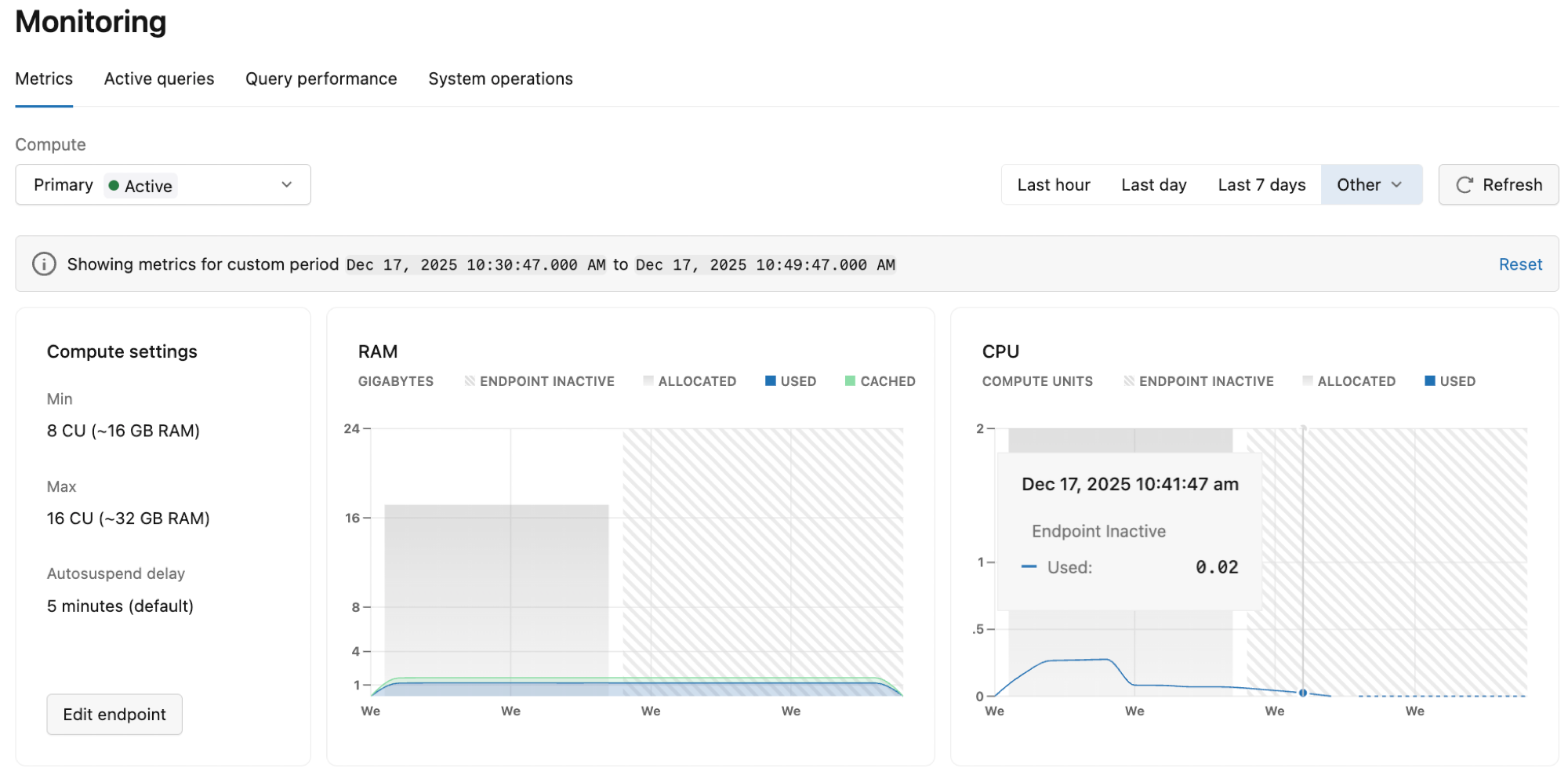
The dashboard displays metrics for the selected branch and compute. Use the drop-down menus to view metrics for a different branch or compute. You can select from predefined time periods (Last hour, Last day, Last 7 days) or choose Other for additional options (Last 3 hours, Last 6 hours, Last 12 hours, Last 2 days, or Custom). Use the Refresh button to update the displayed metrics.
Understanding inactive computes
If graphs are not showing any data, your compute may be inactive due to scale to zero.
When a compute is inactive, metric values drop to 0 because an active compute is required to report data. Inactive periods appear as a diagonal line pattern in the graphs.
If graphs display no data, try selecting a different time period or return later after more usage data has been collected.
RAM
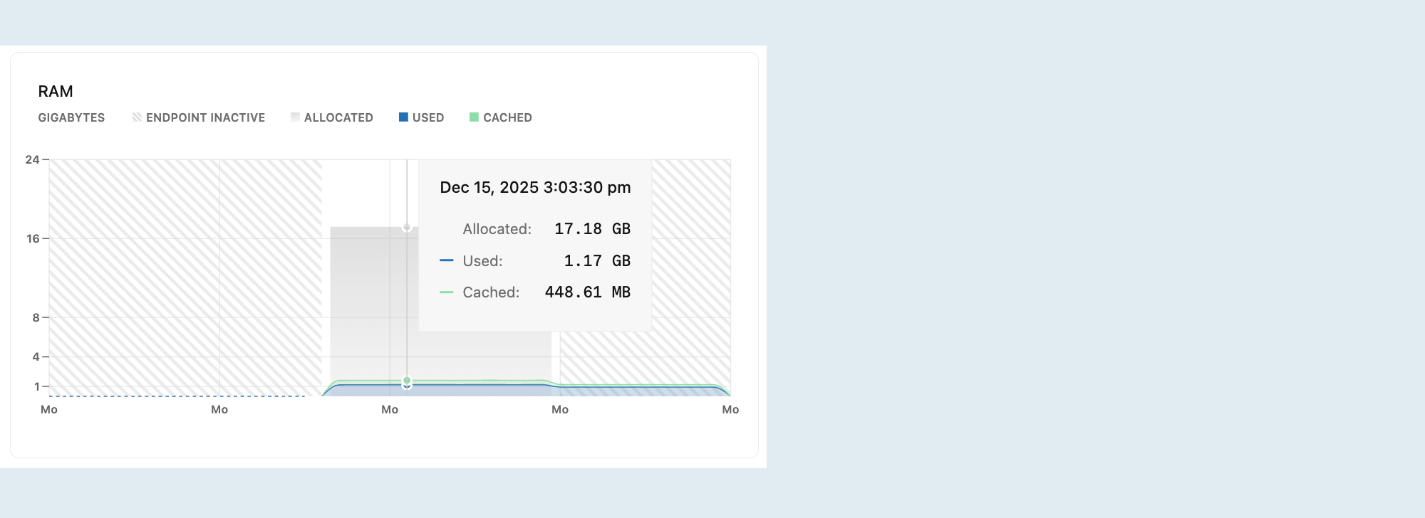
This graph shows allocated RAM and usage over time for the selected compute.
It includes the following metrics:
Allocated: The amount of allocated RAM.
RAM is allocated according to the size of your compute or your autoscaling configuration. With autoscaling, allocated RAM increases and decreases as your compute scales up and down in response to load. If scale to zero is enabled and your compute transitions to an idle state after inactivity, allocated RAM drops to 0.
Used: The amount of RAM used.
The graph plots a line showing RAM usage. If the line regularly reaches the maximum allocated RAM, consider increasing your compute size. For compute size options, see Compute sizing.
Cached: The amount of data cached in memory by previous queries and operations.
CPU
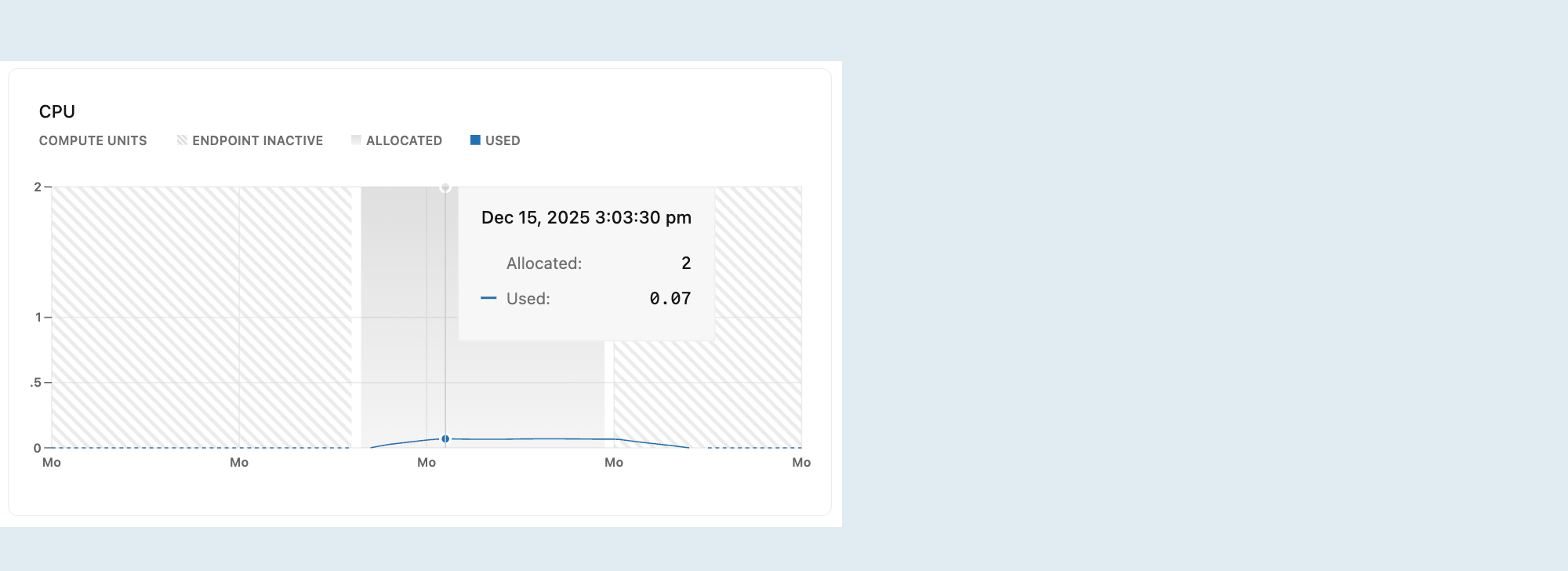
This graph shows allocated CPU and usage over time for the selected compute.
Allocated: The amount of allocated CPU.
CPU is allocated according to the size of your compute or your autoscaling configuration. With autoscaling, allocated CPU increases and decreases as your compute scales up and down in response to load. If scale to zero is enabled and your compute transitions to an idle state after inactivity, allocated CPU drops to 0.
Used: The amount of CPU used, in Compute Units (CU).
If the plotted line regularly reaches the maximum allocated CPU, consider increasing your compute size. For compute size options, see Compute sizing.
Connections count
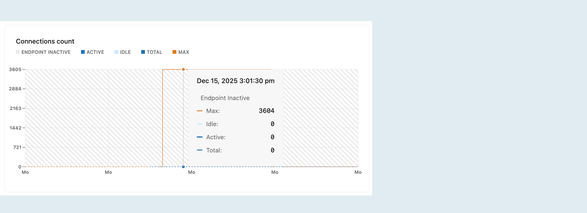
The Connections count graph shows the maximum number of connections, the number of idle connections, the number of active connections, and the total number of connections over time for the selected compute.
Active: The number of active connections for the selected compute.
Monitoring active connections helps you understand your database workload. If the number of active connections is consistently high, your database may be under heavy load, which could lead to performance issues such as slow query response times.
Idle: The number of idle connections for the selected compute.
Idle connections are open but not currently in use. While a few idle connections are generally harmless, a large number can consume unnecessary resources, leaving less room for active connections and potentially affecting performance. Identifying and closing unnecessary idle connections can help free up resources.
Total: The sum of active and idle connections for the selected compute.
Max: The maximum number of simultaneous connections allowed for your compute size.
The Max line helps you visualize how close you are to reaching your connection limit. When your Total connections approach the Max line, consider:
- Increasing your compute size to allow for more connections
- Optimizing your application's connection management (using connection pooling, closing unused connections promptly, and avoiding long-lived idle connections)
The connection limit is defined by the Postgres max_connections setting and is determined by your compute size configuration. For a complete list of max connections by compute size, see Compute specifications.
Database size
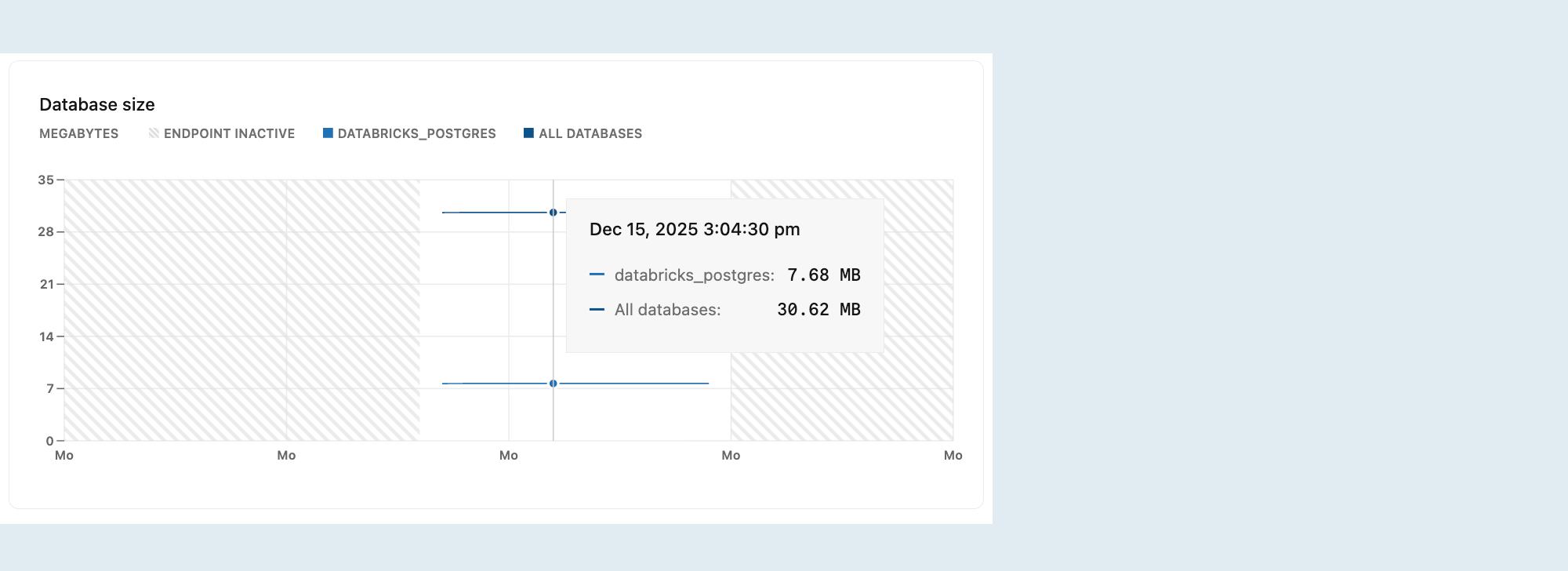
The Database size graph shows the size of your actual data for the selected database or all databases on the selected branch.
When a database reaches its storage quota, write performance drops.
Logical size represents the size of your data as reported by Postgres, including tables and indexes.
Database size metrics are only displayed while your compute is active. When your compute is idle, database size values are not reported, and the graph shows zero even though data may be present.
Deadlocks
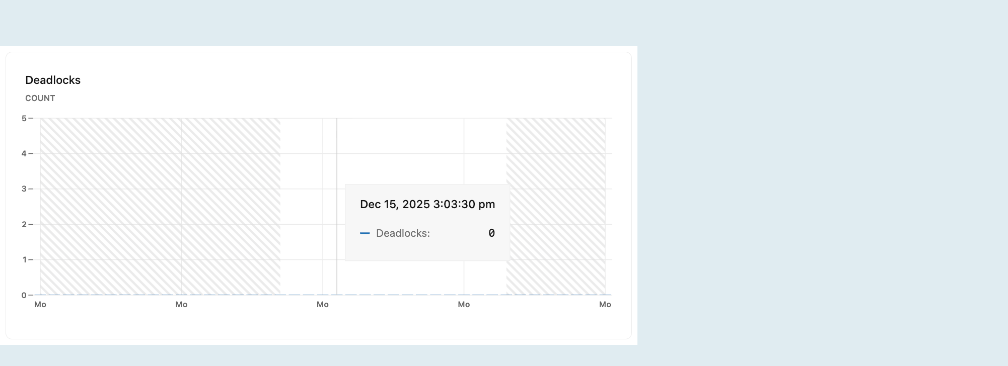
The Deadlocks graph shows a count of deadlocks over time.
Deadlocks occur when two or more transactions simultaneously block each other by holding resources the other transactions need, creating a cycle of dependencies that prevents any transaction from proceeding. This can lead to performance issues or application errors. To learn more about deadlocks in Postgres, refer to the PostgreSQL documentation on deadlocks.
Rows
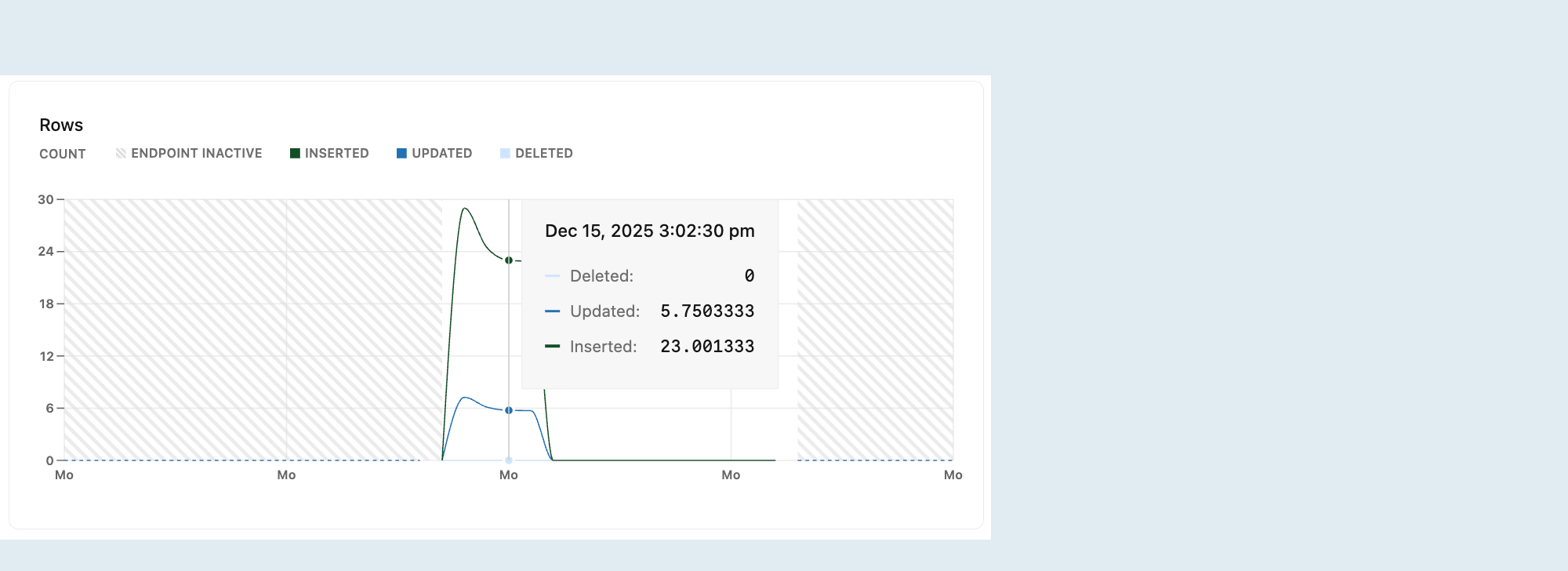
The Rows graph shows the number of rows deleted, updated, and inserted over time. Row metrics reset to zero whenever your compute restarts.
Tracking rows inserted, updated, and deleted over time provides insights into your database's activity patterns. You can use this data to identify trends or irregularities, such as insert spikes or an unusual number of deletions.
Row metrics only capture row-level changes (INSERT, UPDATE, DELETE) and exclude table-level operations such as TRUNCATE.
Replication delay bytes
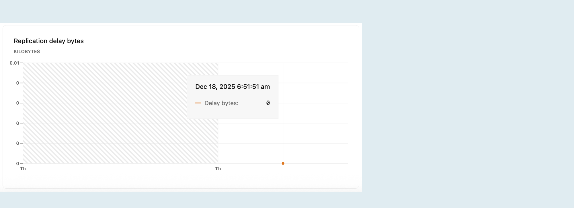
The Replication delay bytes graph shows the total size, in bytes, of data sent from the primary compute but not yet applied on the replica. A larger value indicates a higher backlog of data waiting to be replicated, which may suggest issues with replication throughput or resource availability on the replica.
This graph is only visible when selecting a read replica compute from the Compute drop-down menu. For more information about read replicas, see Read replicas.
Replication delay seconds
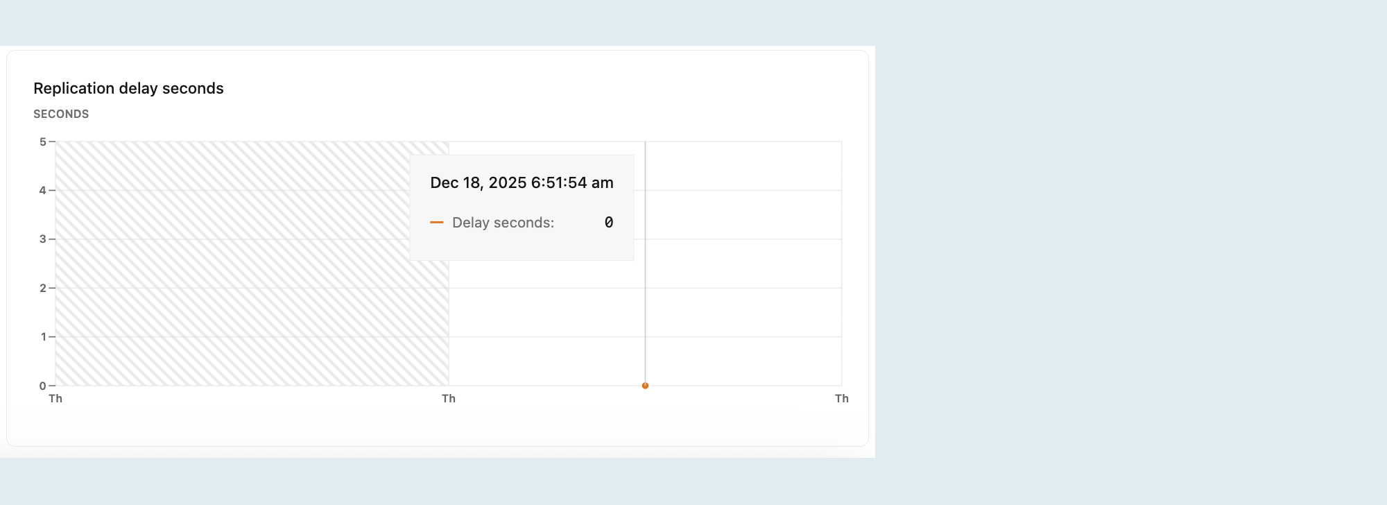
The Replication delay seconds graph shows the time delay, in seconds, between the last transaction committed on the primary compute and the application of that transaction on the replica. A higher value suggests that the replica is behind the primary, potentially due to network latency, high replication load, or resource constraints on the replica.
This graph is only visible when selecting a read replica compute from the Compute drop-down menu. For more information about read replicas, see Read replicas.
Local file cache hit rate
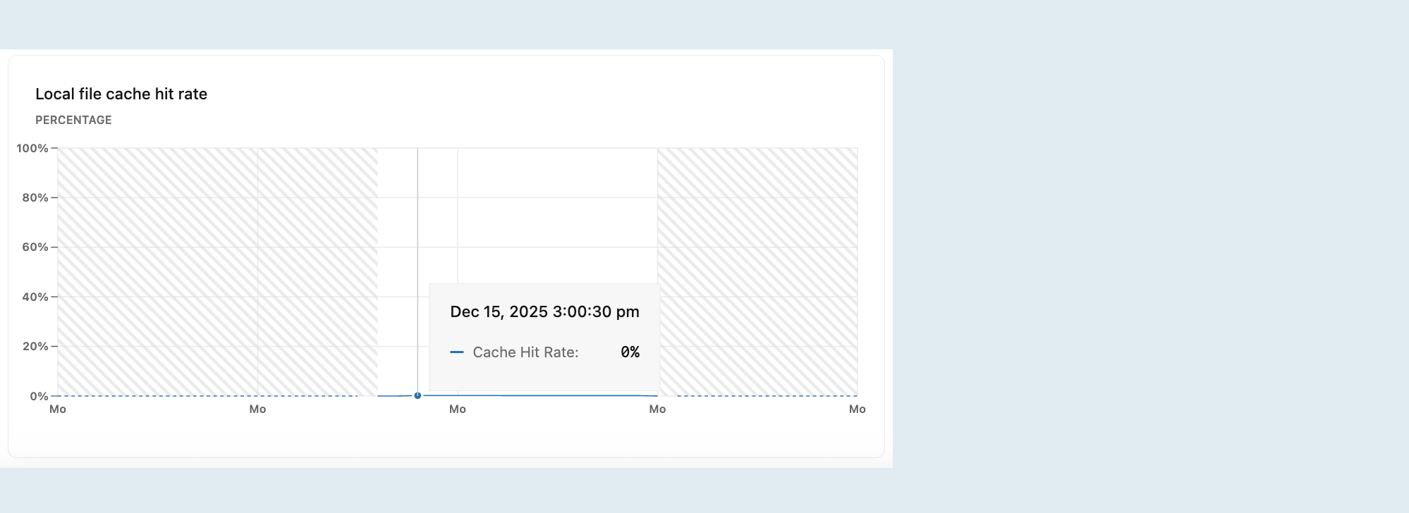
The Local file cache hit rate graph shows the percentage of read requests served from the local file cache. Queries not served from either Postgres shared buffers or the local file cache retrieve data from storage, which is more costly and can result in slower query performance.
For OLTP workloads, aim for a cache hit rate of 99% or better. If your rate is below 99%, your working set may not fit in memory, resulting in slower performance. To improve the cache hit rate, increase your compute size to expand the local file cache. The ideal ratio depends on your workload—workloads with sequential scans of large tables may perform acceptably with a slightly lower ratio.
The local file cache (LFC) is a caching layer that stores frequently accessed data in your compute's local memory. When data is requested, Postgres checks shared buffers first, then the LFC, and finally retrieves from storage if needed. The LFC size scales with your compute—it can use up to 75% of your compute's RAM. For example, a compute with 8 GB RAM has a 6 GB local file cache. For optimal performance, size your compute so that your working set fits within the local file cache.
Working set size
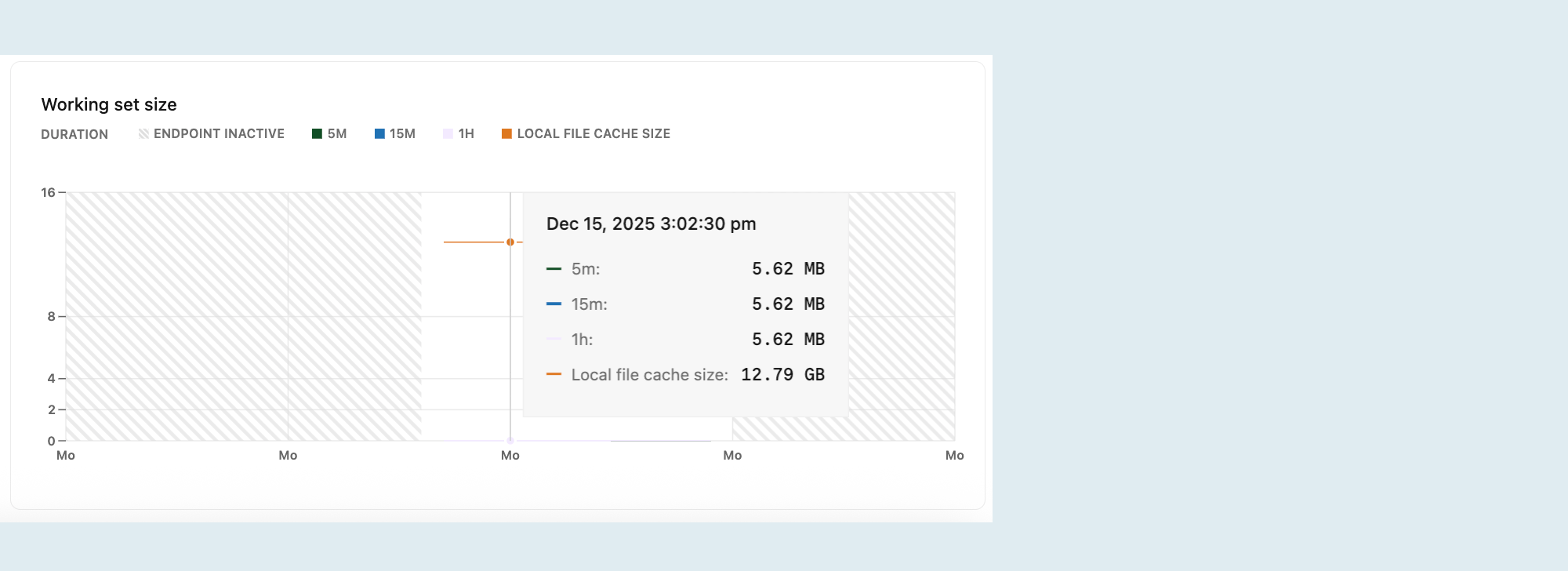
Your working set is the size of the distinct set of Postgres pages (relation data and indexes) accessed in a given time interval. For optimal performance and consistent latency, size your compute so that the working set fits into the local file cache for quick access.
The Working set size graph visualizes the amount of data accessed (calculated as unique pages accessed × page size) over a given interval. The graph displays:
5m (5 minutes): The data accessed in the last 5 minutes.
15m (15 minutes): The data accessed in the last 15 minutes.
1h (1 hour): The data accessed in the last hour.
Local file cache size: The size of the local file cache, determined by the size of your compute. Larger computes have larger caches.
For optimal performance, the local file cache should be larger than your working set size for a given time interval. If your working set size is larger than the local file cache size, increase the maximum size of your compute to improve the cache hit rate and achieve better performance. For compute sizing options and specifications, see Compute specifications.
If your workload pattern doesn't change much over time, compare the 1-hour working set size with the local file cache size and ensure that the working set size is smaller than the local file cache size.