Data profiling metric tables
This page describes the metric tables created by data profiling. For information about the dashboard created by a profile, see Data profiling dashboard.
When a profile runs on a Databricks table, it creates or updates two metric tables: a profile metrics table and a drift metrics table.
- The profile metrics table contains summary statistics for each column and for each combination of time window, slice, and grouping columns. For
InferenceLoganalysis, the analysis table also contains model accuracy metrics. - The drift metrics table contains statistics that track changes in distribution for a metric. Drift tables can be used to visualize or alert on changes in the data instead of specific values. The following types of drift are computed:
- Consecutive drift compares a window to the previous time window. Consecutive drift is only calculated if a consecutive time window exists after aggregation according to the specified granularities.
- Baseline drift compares a window to the baseline distribution determined by the baseline table. Baseline drift is only calculated if a baseline table is provided.
Where metric tables are located
Metric tables are saved to {output_schema}.{table_name}_profile_metrics and {output_schema}.{table_name}_drift_metrics, where:
{output_schema}is the catalog and schema specified byoutput_schema_name.{table_name}is the name of the table being profiled.
How profile statistics are computed
Each statistic and metric in the metric tables is computed for a specified time interval (called a “window”). For Snapshot analysis, the time window is a single point in time corresponding to the time the metric was refreshed. For TimeSeries and InferenceLog analysis, the time window is based on the granularities specified in create_monitor and the values in the timestamp_col specified in the profile_type argument.
Metrics are always computed for the entire table. In addition, if you provide a slicing expression, metrics are computed for each data slice defined by a value of the expression.
For example:
slicing_exprs=["col_1", "col_2 > 10"]
generates the following slices: one for col_2 > 10, one for col_2 <= 10, and one for each unique value in col1.
Slices are identified in the metrics tables by the column names slice_key and slice_value. In this example, one slice key would be “col_2 > 10” and the corresponding values would be “true” and “false”. The entire table is equivalent to slice_key = NULL and slice_value = NULL. Slices are defined by a single slice key.
Metrics are computed for all possible groups defined by the time windows and slice keys and values. In addition, for InferenceLog analysis, metrics are computed for each model id. For details, see Column schemas for generated tables.
Additional statistics for model accuracy (InferenceLog analysis only)
Additional statistics are calculated for InferenceLog analysis.
- Model quality is calculated if both
label_colandprediction_colare provided. - Slices are automatically created based on the distinct values of
model_id_col. - For classification models, fairness and bias statistics are calculated for slices that have a Boolean value.
Query analysis and drift metrics tables
You can query the metrics tables directly. The following example is based on InferenceLog analysis:
SELECT
  window.start, column_name, count, num_nulls, distinct_count, frequent_items
FROM census_monitor_db.adult_census_profile_metrics
WHERE model_id = 1    — Constrain to version 1
  AND slice_key IS NULL    — look at aggregate metrics over the whole data
  AND column_name = "income_predicted"
ORDER BY window.start
Column schemas for generated tables
For each column in the primary table, the metrics tables contain one row for each combination of grouping columns. The column associated with each row is shown in the column column_name.
For metrics based on more than one column such as model accuracy metrics, column_name is set to :table.
For profile metrics, the following grouping columns are used:
- time window
- granularity (
TimeSeriesandInferenceLoganalysis only) - log type - input table or baseline table
- slice key and value
- model id (
InferenceLoganalysis only)
For drift metrics, the following additional grouping columns are used:
- comparison time window
- drift type (comparison to previous window or comparison to baseline table)
The schemas of the metric tables are shown below, and are also shown in the data profiling API reference documentation.
Profile metrics table schema
The following table shows the schema of the profile metrics table. Where a metric is not applicable to a row, the corresponding cell is null.
Column name | Type | Description |
|---|---|---|
Grouping columns | ||
window | Struct. See [1] below. | Time window. |
granularity | string | Window duration, set by |
model_id_col | string | Optional. Only used for |
log_type | string | Table used to calculate metrics. BASELINE or INPUT. |
slice_key | string | Slice expression. NULL for default, which is all data. |
slice_value | string | Value of the slicing expression. |
column_name | string | Name of column in primary table. |
data_type | string | Spark data type of |
logging_table_commit_version | int | Ignore. |
monitor_version | bigint | Version of the profile configuration used to calculate the metrics in the row. See [3] below for details. |
Metrics columns - summary statistics | ||
count | bigint | Number of non-null values. |
num_nulls | bigint | Number of null values in |
avg | double | Arithmetic mean of the column, ignoring nulls. |
quantiles |
| Array of 1000 quantiles. See [4] below. |
distinct_count | bigint | Approximate number of distinct values in |
min | double | Minimum value in |
max | double | Maximum value in |
stddev | double | Standard deviation of |
num_zeros | bigint | Number of zeros in |
num_nan | bigint | Number of NaN values in |
min_size | double | Minimum size of arrays or structures in |
max_size | double | Maximum size of arrays or structures in |
avg_size | double | Average size of arrays or structures in |
min_len | double | Minimum length of string and binary values in |
max_len | double | Maximum length of string and binary values in |
avg_len | double | Average length of string and binary values in |
frequent_items | Struct. See [1] below. | Top 100 most frequently occurring items. |
non_null_columns |
| List of columns with at least one non-null value. |
median | double | Median value of |
percent_null | double | Percent of null values in |
percent_zeros | double | Percent of values that are zero in |
percent_distinct | double | Percent of values that are distinct in |
Metrics columns - classification model accuracy [5] | ||
accuracy_score | double | Accuracy of model, calculated as:
Null values are ignored. |
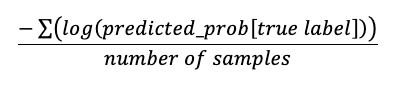
log_loss | double | Log loss for classification problems, calculated as:
Requires |
roc_auc_score | Struct. See [1] below. | ROC AUC score for binary and multi-class classification. Requires |
confusion_matrix | Struct. See [1] below. | |
precision | Struct. See [1] below. | |
recall | Struct. See [1] below. | |
f1_score | Struct. See [1] below. | |
Metrics columns - regression model accuracy [5] | ||
mean_squared_error | double | Mean squared error between |
root_mean_squared_error | double | Root mean squared error between |
mean_average_error | double | Mean average error between |
mean_absolute_percentage_error | double | Mean absolute percentage error between |
r2_score | double | R-squared score between |
Metrics columns - fairness and bias [6] | ||
predictive_parity | double | Measures whether the two groups have equal precision across all predicted classes. |
predictive_equality | double | Measures whether the two groups have equal false positive rate across all predicted classes. |
equal_opportunity | double | Measures whether the two groups have equal recall across all predicted classes. |
statistical_parity | double | Measures whether the two groups have equal acceptance rate. Acceptance rate here is defined as the empirical probability to be predicted as a certain class, across all predicted classes. |

[1] Format of struct for confusion_matrix, precision, recall, f1_score, and roc_auc_score:
Column name | Type |
|---|---|
window |
|
frequent_items |
|
confusion_matrix |
|
precision |
|
recall |
|
f1_score |
|
roc_auc_score |
|
[2] For time series or inference profiles, the profile looks back 30 days from the time the profile is created. Due to this cutoff, the first analysis might include a partial window. For example, the 30 day limit might fall in the middle of a week or month, in which case the full week or month is not included in the calculation. This issue affects only the first window.
[3] The version shown in this column is the version that was used to calculate the statistics in the row and might not be the current version of the profile. Each time you refresh the metrics, the profile attempts to recompute previously calculated metrics using the current profile configuration. The current profile version appears in the profile information returned by the API and Python Client.
[4] Sample code to retrieve the 50th percentile: SELECT element_at(quantiles, int((size(quantiles)+1)/2)) AS p50 ... or SELECT quantiles[500] ... .
[5] Only shown if the profile has InferenceLog analysis type and both label_col and prediction_col are provided.
[6] Only shown if the profile has InferenceLog analysis type and problem_type is classification.
Drift metrics table schema
The following table shows the schema of the drift metrics table. The drift table is only generated if a baseline table is provided, or if a consecutive time window exists after aggregation according to the specified granularities. Where a metric is not applicable to a row, the corresponding cell is null.
Column name | Type | Description |
|---|---|---|
Grouping columns | ||
window |
| Time window. |
window_cmp |
| Comparison window for drift_type |
drift_type | string | BASELINE or CONSECUTIVE. Whether the drift metrics compare to the previous time window or to the baseline table. |
granularity | string | Window duration, set by |
model_id_col | string | Optional. Only used for |
slice_key | string | Slice expression. NULL for default, which is all data. |
slice_value | string | Value of the slicing expression. |
column_name | string | Name of column in primary table. |
data_type | string | Spark data type of |
monitor_version | bigint | Version of the monitor configuration used to calculate the metrics in the row. See [8] below for details. |
Metrics columns - drift | Differences are calculated as current window - comparison window. | |
count_delta | double | Difference in |
avg_delta | double | Difference in |
percent_null_delta | double | Difference in |
percent_zeros_delta | double | Difference in |
percent_distinct_delta | double | Difference in |
non_null_columns_delta |
| Number of columns with any increase or decrease in non-null values. |
chi_squared_test |
| Chi-square test for drift in distribution. Calculated for categorical columns only. |
ks_test |
| KS test for drift in distribution. Calculated for numeric columns only. |
tv_distance | double | Total variation distance for drift in distribution. Calculated for categorical columns only. |
l_infinity_distance | double | L-infinity distance for drift in distribution. Calculated for categorical columns only. |
js_distance | double | Jensen–Shannon distance for drift in distribution. Calculated for categorical columns only. |
wasserstein_distance | double | Drift between two numeric distributions using the Wasserstein distance metric. Calculated for numeric columns only. |
population_stability_index | double | Metric for comparing the drift between two numeric distributions using the population stability index metric. See [9] below for details. Calculated for numeric columns only. |
[7] For time series or inference profiles, the profile looks back 30 days from the time the profile is created. Due to this cutoff, the first analysis might include a partial window. For example, the 30 day limit might fall in the middle of a week or month, in which case the full week or month is not included in the calculation. This issue affects only the first window.
[8] The version shown in this column is the version that was used to calculate the statistics in the row and might not be the current version of the profile. Each time you refresh the metrics, the profile attempts to recompute previously calculated metrics using the current profile configuration. The current profile version appears in the profile information returned by the API and Python Client.
[9] The output of the population stability index is a numeric value that represents how different two distributions are. The range is [0, inf). PSI < 0.1 means no significant population change. PSI < 0.2 indicates moderate population change. PSI >= 0.2 indicates significant population change.