MLOps workflows on Databricks

This article describes how you can use MLOps on the Databricks platform to optimize the performance and long-term efficiency of your machine learning (ML) systems. It includes general recommendations for an MLOps architecture and describes a generalized workflow using the Databricks platform that you can use as a model for your ML development-to-production process. For modifications of this workflow for LLMOps applications, see LLMOps workflows.

For more details, see The Big Book of MLOps.

What is MLOps?

MLOps is a set of processes and automated steps for managing code, data, and models to improve performance, stability, and long-term efficiency of ML systems. It combines DevOps, DataOps, and ModelOps.

ML assets such as code, data, and models are developed in stages that progress from early development stages that do not have tight access limitations and are not rigorously tested, through an intermediate testing stage, to a final production stage that is tightly controlled. The Databricks platform lets you manage these assets on a single platform with unified access control. You can develop data applications and ML applications on the same platform, reducing the risks and delays associated with moving data around.

General recommendations for MLOps

This section includes some general recommendations for MLOps on Databricks with links for more information.

Create a separate environment for each stage

An execution environment is the place where models and data are created or consumed by code. Each execution environment consists of compute instances, their runtimes and libraries, and automated jobs.

Databricks recommends creating separate environments for the different stages of ML code and model development with clearly defined transitions between stages. The workflow described in this article follows this process, using the common names for the stages:

• Development
• Staging
• Production

Other configurations can also be used to meet the specific needs of your organization.

Access control and versioning

Access control and versioning are key components of any software operations process. Databricks recommends the following:

• Use Git for version control. Pipelines and code should be stored in Git for version control. Moving ML logic between stages can then be interpreted as moving code from the development branch, to the staging branch, to the release branch. Use Databricks Git folders to integrate with your Git provider and sync notebooks and source code with Databricks workspaces. Databricks also provides additional tools for Git integration and version control; see Local development tools.
• Store data in a lakehouse architecture using Delta tables. Data should be stored in a lakehouse architecture in your cloud account. Both raw data and feature tables should be stored as Delta tables with access controls to determine who can read and modify them.
• Manage model development with MLflow. You can use MLflow to track the model development process and save code snapshots, model parameters, metrics, and other metadata.
• Use Models in Unity Catalog to manage the model lifecycle. Use Models in Unity Catalog to manage model versioning, governance, and deployment status.

Deploy code, not models

In most situations, Databricks recommends that during the ML development process, you promote code, rather than models, from one environment to the next. Moving project assets this way ensures that all code in the ML development process goes through the same code review and integration testing processes. It also ensures that the production version of the model is trained on production code. For a more detailed discussion of the options and trade-offs, see Model deployment patterns.

Recommended MLOps workflow

The following sections describe a typical MLOps workflow, covering each of the three stages: development, staging, and production.

This section uses the terms “data scientist” and “ML engineer” as archetypal personas; specific roles and responsibilities in the MLOps workflow will vary between teams and organizations.

Development stage

The focus of the development stage is experimentation. Data scientists develop features and models and run experiments to optimize model performance. The output of the development process is ML pipeline code that can include feature computation, model training, inference, and monitoring.

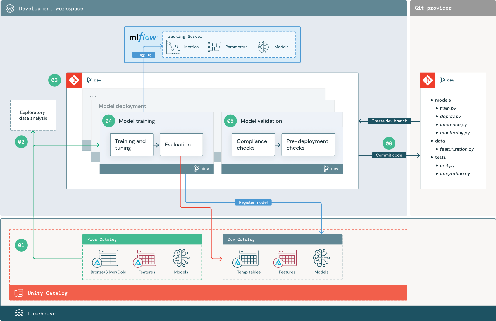
The numbered steps correspond to the numbers shown in the diagram.

1. Data sources

The development environment is represented by the dev catalog in Unity Catalog. Data scientists have read-write access to the dev catalog as they create temporary data and feature tables in the development workspace. Models created in the development stage are registered to the dev catalog.

Ideally, data scientists working in the development workspace also have read-only access to production data in the prod catalog. Allowing data scientists read access to production data, inference tables, and metric tables in the prod catalog enables them to analyze current production model predictions and performance. Data scientists should also be able to load production models for experimentation and analysis.

If it is not possible to grant read-only access to the prod catalog, a snapshot of production data can be written to the dev catalog to enable data scientists to develop and evaluate project code.

2. Exploratory data analysis (EDA)

Data scientists explore and analyze data in an interactive, iterative process using notebooks. The goal is to assess whether the available data has the potential to solve the business problem. In this step, the data scientist begins identifying data preparation and featurization steps for model training. This ad hoc process is generally not part of a pipeline that will be deployed in other execution environments.

AutoML accelerates this process by generating baseline models for a dataset. AutoML performs and records a set of trials and provides a Python notebook with the source code for each trial run, so you can review, reproduce, and modify the code. AutoML also calculates summary statistics on your dataset and saves this information in a notebook that you can review.

3. Code

The code repository contains all of the pipelines, modules, and other project files for an ML project. Data scientists create new or updated pipelines in a development (“dev”) branch of the project repository. Starting from EDA and the initial phases of a project, data scientists should work in a repository to share code and track changes.

4. Train model (development)

Data scientists develop the model training pipeline in the development environment using tables from the dev or prod catalogs.

This pipeline includes 2 tasks:

• Training and tuning. The training process logs model parameters, metrics, and artifacts to the MLflow Tracking server. After training and tuning hyperparameters, the final model artifact is logged to the tracking server to record a link between the model, the input data it was trained on, and the code used to generate it.

• Evaluation. Evaluate model quality by testing on held-out data. The results of these tests are logged to the MLflow Tracking server. The purpose of evaluation is to determine if the newly developed model performs better than the current production model. Given sufficient permissions, any production model registered to the prod catalog can be loaded into the development workspace and compared against a newly trained model.

  If your organization's governance requirements include additional information about the model, you can save it using MLflow tracking. Typical artifacts are plain text descriptions and model interpretations such as plots produced by SHAP. Specific governance requirements may come from a data governance officer or business stakeholders.

The output of the model training pipeline is an ML model artifact stored in the MLflow Tracking server for the development environment. If the pipeline is executed in the staging or production workspace, the model artifact is stored in the MLflow Tracking server for that workspace.

When the model training is complete, register the model to Unity Catalog. Set up your pipeline code to register the model to the catalog corresponding to the environment that the model pipeline was executed in; in this example, the dev catalog.

With the recommended architecture, you deploy a multitask Databricks workflow in which the first task is the model training pipeline, followed by model validation and model deployment tasks. The model training task yields a model URI that the model validation task can use. You can use task values to pass this URI to the model.

5. Validate and deploy model (development)

In addition to the model training pipeline, other pipelines such as model validation and model deployment pipelines are developed in the development environment.

• Model validation. The model validation pipeline takes the model URI from the model training pipeline, loads the model from Unity Catalog, and runs validation checks.

  Validation checks depend on the context. They can include fundamental checks such as confirming format and required metadata, and more complex checks that might be required for highly regulated industries, such as predefined compliance checks and confirming model performance on selected data slices.

  The primary function of the model validation pipeline is to determine whether a model should proceed to the deployment step. If the model passes pre-deployment checks, it can be assigned the “Challenger” alias in Unity Catalog. If the checks fail, the process ends. You can configure your workflow to notify users of a validation failure. See Add notifications on a job.

• Model deployment. The model deployment pipeline typically either directly promotes the newly trained “Challenger” model to “Champion” status using an alias update, or facilitates a comparison between the existing “Champion” model and the new “Challenger” model. This pipeline can also set up any required inference infrastructure, such as Model Serving endpoints. For a detailed discussion of the steps involved in the model deployment pipeline, see Production.

6. Commit code

After developing code for training, validation, deployment and other pipelines, the data scientist or ML engineer commits the dev branch changes into source control.

Staging stage

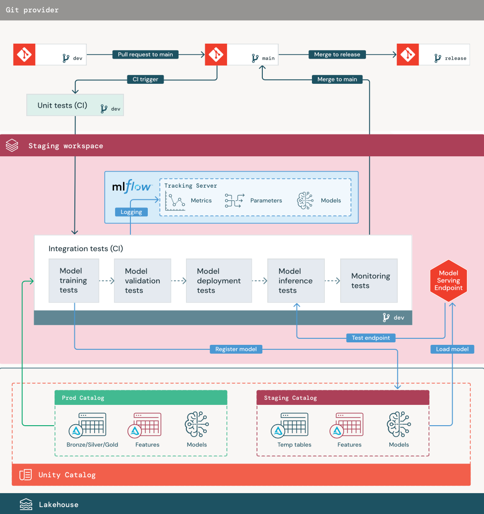
The focus of this stage is testing the ML pipeline code to ensure it is ready for production. All of the ML pipeline code is tested in this stage, including code for model training as well as feature engineering pipelines, inference code, and so on.

ML engineers create a CI pipeline to implement the unit and integration tests run in this stage. The output of the staging process is a release branch that triggers the CI/CD system to start the production stage.

1. Data

The staging environment should have its own catalog in Unity Catalog for testing ML pipelines and registering models to Unity Catalog. This catalog is shown as the “staging” catalog in the diagram. Assets written to this catalog are generally temporary and only retained until testing is complete. The development environment may also require access to the staging catalog for debugging purposes.

2. Merge code

Data scientists develop the model training pipeline in the development environment using tables from the development or production catalogs.

• Pull request. The deployment process begins when a pull request is created against the main branch of the project in source control.

• Unit tests (CI). The pull request automatically builds source code and triggers unit tests. If unit tests fail, the pull request is rejected.

  Unit tests are part of the software development process and are continuously executed and added to the codebase during the development of any code. Running unit tests as part of a CI pipeline ensures that changes made in a development branch do not break existing functionality.

3. Integration tests (CI)

The CI process then runs the integration tests. Integration tests run all pipelines (including feature engineering, model training, inference, and monitoring) to ensure that they function correctly together. The staging environment should match the production environment as closely as is reasonable.

If you are deploying an ML application with real-time inference, you should create and test serving infrastructure in the staging environment. This involves triggering the model deployment pipeline, which creates a serving endpoint in the staging environment and loads a model.

To reduce the time required to run integration tests, some steps can trade off between fidelity of testing and speed or cost. For example, if models are expensive or time-consuming to train, you might use small subsets of data or run fewer training iterations. For model serving, depending on production requirements, you might do full-scale load testing in integration tests, or you might just test small batch jobs or requests to a temporary endpoint.

4. Merge to staging branch

If all tests pass, the new code is merged into the main branch of the project. If tests fail, the CI/CD system should notify users and post results on the pull request.

You can schedule periodic integration tests on the main branch. This is a good idea if the branch is updated frequently with concurrent pull requests from multiple users.

5. Create a release branch

After CI tests have passed and the dev branch is merged into the main branch, the ML engineer creates a release branch, which triggers the CI/CD system to update production jobs.

Production stage

ML engineers own the production environment where ML pipelines are deployed and executed. These pipelines trigger model training, validate and deploy new model versions, publish predictions to downstream tables or applications, and monitor the entire process to avoid performance degradation and instability.

Data scientists typically do not have write or compute access in the production environment. However, it is important that they have visibility to test results, logs, model artifacts, production pipeline status, and monitoring tables. This visibility allows them to identify and diagnose problems in production and to compare the performance of new models to models currently in production. You can grant data scientists read-only access to assets in the production catalog for these purposes.

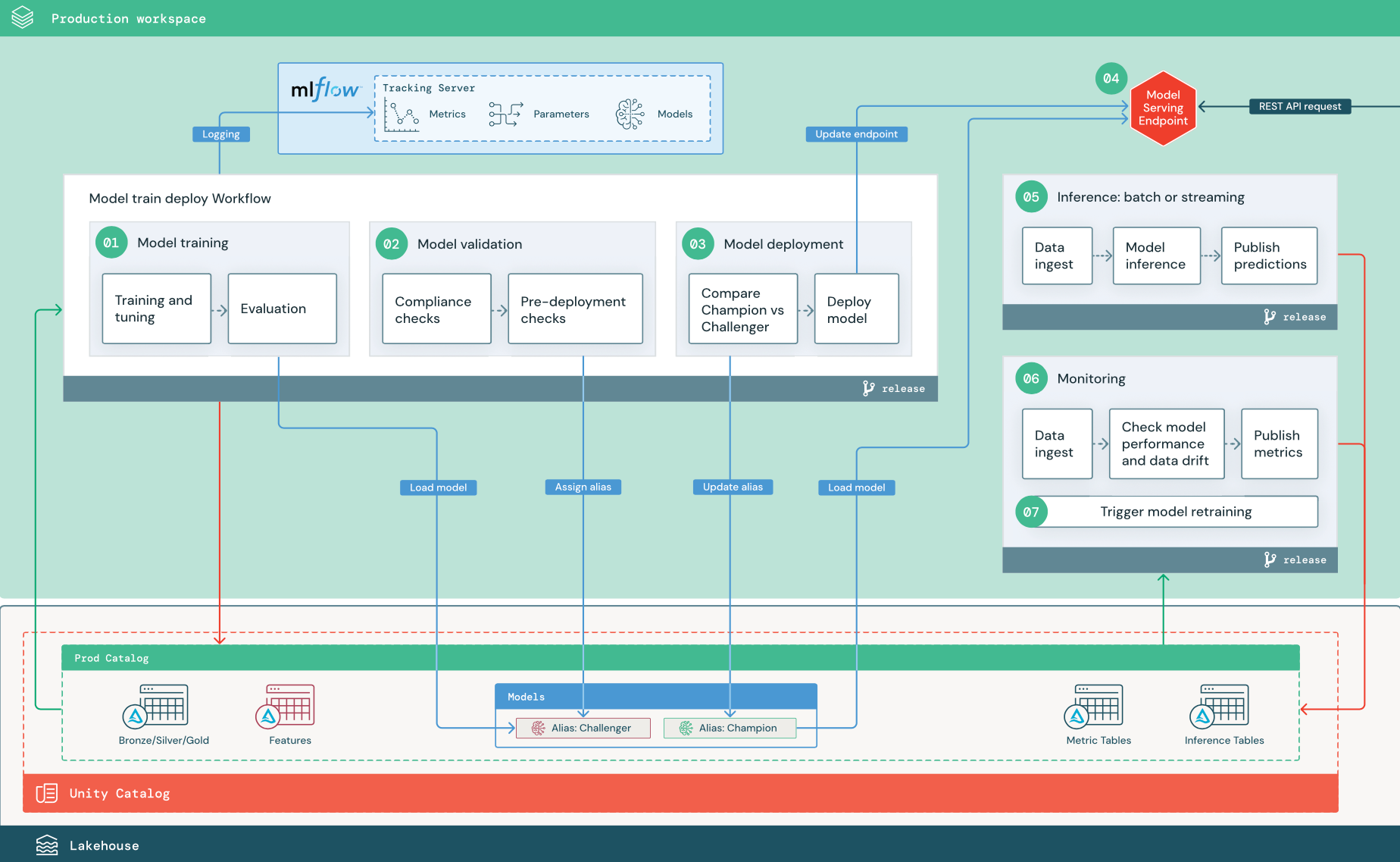
The numbered steps correspond to the numbers shown in the diagram.

1. Train model

This pipeline can be triggered by code changes or by automated retraining jobs. In this step, tables from the production catalog are used for the following steps.

• Training and tuning. During the training process, logs are recorded to the production environment MLflow Tracking server. These logs include model metrics, parameters, tags, and the model itself. If you use feature tables, the model is logged to MLflow using the Databricks Feature Store client, which packages the model with feature lookup information that is used at inference time.

  During development, data scientists may test many algorithms and hyperparameters. In the production training code, it's common to consider only the top-performing options. Limiting tuning in this way saves time and can reduce the variance from tuning in automated retraining.

  If data scientists have read-only access to the production catalog, they may be able to determine the optimal set of hyperparameters for a model. In this case, the model training pipeline deployed in production can be executed using the selected set of hyperparameters, typically included in the pipeline as a configuration file.

• Evaluation. Model quality is evaluated by testing on held-out production data. The results of these tests are logged to the MLflow tracking server. This step uses the evaluation metrics specified by data scientists in the development stage. These metrics may include custom code.

• Register model. When model training is complete, the model artifact is saved as a registered model version at the specified model path in the production catalog in Unity Catalog. The model training task yields a model URI that the model validation task can use. You can use task values to pass this URI to the model.

2. Validate model

This pipeline uses the model URI from Step 1 and loads the model from Unity Catalog. It then executes a series of validation checks. These checks depend on your organization and use case, and can include things like basic format and metadata validations, performance evaluations on selected data slices, and compliance with organizational requirements such as compliance checks for tags or documentation.

If the model successfully passes all validation checks, you can assign the “Challenger” alias to the model version in Unity Catalog. If the model does not pass all validation checks, the process exits and users can be automatically notified. You can use tags to add key-value attributes depending on the outcome of these validation checks. For example, you could create a tag “model_validation_status” and set the value to “PENDING” as the tests execute, and then update it to “PASSED” or “FAILED” when the pipeline is complete.

Because the model is registered to Unity Catalog, data scientists working in the development environment can load this model version from the production catalog to investigate if the model fails validation. Regardless of the outcome, results are recorded to the registered model in the production catalog using annotations to the model version.

3. Deploy model

Like the validation pipeline, the model deployment pipeline depends on your organization and use case. This section assumes that you have assigned the newly validated model the “Challenger” alias, and that the existing production model has been assigned the “Champion” alias. The first step before deploying the new model is to confirm that it performs at least as well as the current production model.

• Compare “CHALLENGER” to “CHAMPION” model. You can perform this comparison offline or online. An offline comparison evaluates both models against a held-out data set and tracks results using the MLflow Tracking server. For real-time model serving, you might want to perform longer running online comparisons, such as A/B tests or a gradual rollout of the new model. If the “Challenger” model version performs better in the comparison, it replaces the current “Champion” alias.

  Mosaic AI Model Serving and Databricks Lakehouse Monitoring allow you to automatically collect and monitor inference tables that contain request and response data for an endpoint.

  If there is no existing “Champion” model, you might compare the “Challenger” model to a business heuristic or other threshold as a baseline.

  The process described here is fully automated. If manual approval steps are required, you can set those up using workflow notifications or CI/CD callbacks from the model deployment pipeline.

• Deploy model. Batch or streaming inference pipelines can be set up to use the model with the “Champion” alias. For real-time use cases, you must set up the infrastructure to deploy the model as a REST API endpoint. You can create and manage this endpoint using Mosaic AI Model Serving. If an endpoint is already in use for the current model, you can update the endpoint with the new model. Mosaic AI Model Serving executes a zero-downtime update by keeping the existing configuration running until the new one is ready.

4. Model Serving

When configuring a Model Serving endpoint, you specify the name of the model in Unity Catalog and the version to serve. If the model version was trained using features from tables in Unity Catalog, the model stores the dependencies for the features and functions. Model Serving automatically uses this dependency graph to look up features from appropriate online stores at inference time. This approach can also be used to apply functions for data preprocessing or to compute on-demand features during model scoring.

You can create a single endpoint with multiple models and specify the endpoint traffic split between those models, allowing you to conduct online “Champion” versus “Challenger” comparisons.

5. Inference: batch or streaming

The inference pipeline reads the latest data from the production catalog, executes functions to compute on-demand features, loads the “Champion” model, scores the data, and returns predictions. Batch or streaming inference is generally the most cost-effective option for higher throughput, higher latency use cases. For scenarios where low-latency predictions are required, but predictions can be computed offline, these batch predictions can be published to an online key-value store such as DynamoDB or Cosmos DB.

The registered model in Unity Catalog is referenced by its alias. The inference pipeline is configured to load and apply the “Champion” model version. If the “Champion” version is updated to a new model version, the inference pipeline automatically uses the new version for its next execution. In this way the model deployment step is decoupled from inference pipelines.

Batch jobs typically publish predictions to tables in the production catalog, to flat files, or over a JDBC connection. Streaming jobs typically publish predictions either to Unity Catalog tables or to message queues like Apache Kafka.

6. Lakehouse Monitoring

Lakehouse Monitoring monitors statistical properties, such as data drift and model performance, of input data and model predictions. You can create alerts based on these metrics or publish them in dashboards.

• Data ingestion. This pipeline reads in logs from batch, streaming, or online inference.
• Check accuracy and data drift. The pipeline computes metrics about the input data, the model's predictions, and the infrastructure performance. Data scientists specify data and model metrics during development, and ML engineers specify infrastructure metrics. You can also define custom metrics with Lakehouse Monitoring.
• Publish metrics and set up alerts. The pipeline writes to tables in the production catalog for analysis and reporting. You should configure these tables to be readable from the development environment so data scientists have access for analysis. You can use Databricks SQL to create monitoring dashboards to track model performance, and set up the monitoring job or the dashboard tool to issue a notification when a metric exceeds a specified threshold.
• Trigger model retraining. When monitoring metrics indicate performance issues or changes in the input data, the data scientist may need to develop a new model version. You can set up SQL alerts to notify data scientists when this happens.

7. Retraining

This architecture supports automatic retraining using the same model training pipeline above. Databricks recommends beginning with scheduled, periodic retraining and moving to triggered retraining when needed.

• Scheduled. If new data is available on a regular basis, you can create a scheduled job to run the model training code on the latest available data. See Automating jobs with schedules and triggers
• Triggered. If the monitoring pipeline can identify model performance issues and send alerts, it can also trigger retraining. For example, if the distribution of incoming data changes significantly or if the model performance degrades, automatic retraining and redeployment can boost model performance with minimal human intervention. This can be achieved through a SQL alert to check whether a metric is anomalous (for example, check drift or model quality against a threshold). The alert can be configured to use a webhook destination, which can subsequently trigger the training workflow.

If the retraining pipeline or other pipelines exhibit performance issues, the data scientist may need to return to the development environment for additional experimentation to address the issues.