Dashboard relationships
This feature is in Public Preview.
Dashboard relationships let you model the join logic between your datasets in AI/BI dashboards, so you can build multi-fact, multi-grain data models and reusable cross-dataset measures without pre-joining data in SQL. You model the relationship once, then use it across every visualization in the dashboard.
What problem do relationships solve?
Before relationships, an author who wanted to join metrics from multiple fact tables (for example, orders.revenue and shipments.cost), grouped by region, had to pre-join both fact tables to the region dimension and aggregate carefully to avoid fan-out, the row duplication that happens when a join multiplies rows instead of matching them one-to-one. That join logic lived in SQL, duplicated across every dataset that needed it.
With relationships, the author defines the join once. The query engine decides what to join at runtime, based on the fields in the visualization. There's no fan-out, double-counting, or duplicated SQL.
How do dashboard relationships work?
You define a relationship between two dashboard datasets by choosing a join field in each and setting the cardinality, such as many-to-one from a fact table to a dimension. The related datasets then form a traversable graph, and the query engine resolves the joins each visualization needs at query time, so filters and measures flow across connected datasets without pre-joining data in SQL.
A model can span several fact tables that meet at shared dimensions, and a dimension can snowflake out to further dimensions. Figure 1 shows a model with three fact tables joined through four shared dimensions, two of which snowflake one level further.
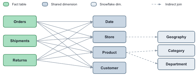
Figure 1. A dashboard relationship model spans multiple fact tables joined through shared dimensions, with some dimensions snowflaked one level further. Even a snowflaked dimension like Geography stays reachable from every connected fact table.
To create relationships and cross-dataset measures, see Create dashboard relationships.
What data models are supported?
Dashboard relationships perform query-time joins between tables based on the specified cardinality of the relationship. You can join fact tables through a conformed dimension (a dimension shared by more than one fact table), but not directly to each other through many-to-many joins.
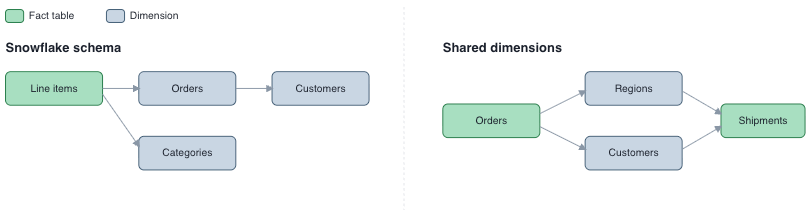
The following table describes the supported and unsupported patterns, and how to resolve unsupported patterns when they occur:
Pattern | Supported | What it looks like | Resolution |
|---|---|---|---|
Snowflake schema | ✅ Yes | A fact table joins a chain of dimensions, for example | None needed |
Shared dimensions | ✅ Yes | Two fact tables join the same conformed dimension, for example | None needed |
Ambiguous join path | ❌ No | A dimension reachable from one fact table by more than one route, for example | Alias one route, for example |
Cyclic relationship | ❌ No | A closed loop of joins with no single unambiguous path, for example | Alias one table in the loop to break the cycle |
How do I resolve ambiguous and cyclic join paths?
Aliasing works because each aliased copy of a table is a distinct node in the graph, so every join path leads to exactly one target. The two unsupported patterns each create a different kind of duplicate path, and aliasing removes it.
An ambiguous join path happens when a fact table can reach the same dimension through more than one route. For example, Orders reaches Country both through Regions and through Customers, so a query that groups orders by country has two candidate joins and no way to choose between them. To resolve it, alias the dimension once per route, such as Country (region) and Country (customer). Each route then points at its own copy, so a field like customer country resolves to exactly one path.
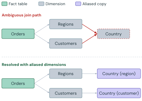
Figure 2. Aliasing the shared dimension gives each route its own target, so the join path is unambiguous.
A cyclic relationship is a closed loop of joins. If Orders joins Regions, Regions joins Customers, and Customers joins back to Orders, the loop gives the query engine no unambiguous place to start or stop, so it can't resolve the joins. To resolve it, alias one table in the loop to break it into a single path the query engine can follow from end to end. In Figure 3, A, B, and C stand for any three tables in such a loop, and A′ is the alias that breaks it.
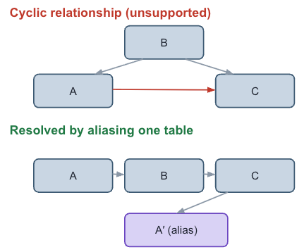
Figure 3. Aliasing one table in the loop breaks the cycle into a single traversable path.
How do cross-dataset measures work?
When fact tables share a conformed dimension, you can define a measure once at the model level and have it draw on more than one fact table. The query engine aggregates each fact table independently and combines the results at the shared dimension, so the measure stays correct no matter which fields a viewer adds to the visualization.
For example, with Orders, Shipments, and Returns joined through shared dimensions, you could define cross-dataset measures like these at the model level:
Net Revenue      = SUM(Orders.revenue) - SUM(Returns.refund)
Fulfillment Rate = SUM(Shipments.units) / SUM(Orders.units)
Return Rate      = SUM(Returns.units) / SUM(Orders.units)
Each of these draws on two fact tables at once, without fan-out or double-counting. Figure 1 shows the shared dimensions this relies on, where three fact tables meet at four conformed dimensions.
Why field order matters
The first field you add sets the root, the table every other field is resolved against. From that root, three kinds of fields behave differently:
Field type | Reachable from a non-root table? |
|---|---|
Field (dimension) | Yes, through any many-to-one chain, however many hops |
Measure (aggregate) | Yes, it aggregates independently, then joins at the shared dimension |
Native column (unaggregated) | No, unless that fact table is the root |
So starting from orders revenue makes customer region and shipments cost both available, but not ship mode: a raw column on Shipments, unreachable because Shipments isn't the root. Start from ship mode instead, and the root flips, so now Shipments' own columns are available too.
How do dashboard relationships compare to metric views?
Both can model the same join graph, but they solve different problems:
- Metric views are fixed grain. You query them directly with SQL, and they're a good fit for star and snowflake schemas.
- Dashboard relationships are dynamic grain. They let you mix and match fields and measures from any table across the semantic graph, so they're a better fit for modeling across multiple fact tables.
A dashboard relationship graph can include metric views as nodes, with relationships as the edges that connect them. The metric view handles the single-grain logic, and relationships handle the multi-fact layer on top.
Aspect | Dashboard relationships | Metric views |
|---|---|---|
Scope | A single dashboard | Unity Catalog, shared across dashboards, Genie Agents, and other tools |
Best for | Prototyping, dashboard-specific analysis, iterating quickly | Metrics that need to be governed and reused consistently |
Creates a UC object | No | Yes |
If you start with a dashboard relationship and later need the same model governed and shared, you can promote it to a metric view. See Unity Catalog metric views and Export to a Unity Catalog metric view. For a broader comparison of all the data modeling options available in AI/BI dashboards, see Choose the right approach.
What is the difference between fixed grain and dynamic grain?
Granularity affects which fields you can select and the grain at which they're expressed. A metric view locks a table at a fixed granularity, such as customer-level, while relationships are dynamic, based on the fields used in the dashboard, such as customer-, order-, or shipment-level.
The difference comes down to the root. A metric view bakes the root into the dimension at definition time: Customer is always the root, so every query groups by Customer, and the field picker only ever offers Customer as a grouping field, even though it still pulls measures from any connected fact table. Dashboard relationships choose the root per query instead: either Orders or Shipments can serve as the root, depending on whichever field you add first, so the field picker lets you group by any of the connected tables rather than just the dimension.
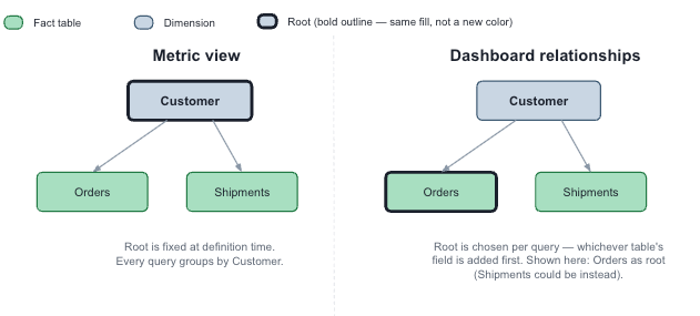
Figure 4. The root is fixed in a metric view but chosen per query in a dashboard relationship.
Despite that difference, both share the same underlying limit: you still can't group one fact table's measure by another fact table's column directly, because the two only meet at the shared dimension.
Why are dashboard relationships scoped to a dashboard?
Support for relationships in Unity Catalog is in progress.