Custom visualizations in AI/BI dashboards
This feature is in Public Preview.
Custom visualizations let you customize charts in AI/BI dashboards beyond the built-in visualization types. Custom visualizations use the Vega-Lite library to render charts from a JSON specification.
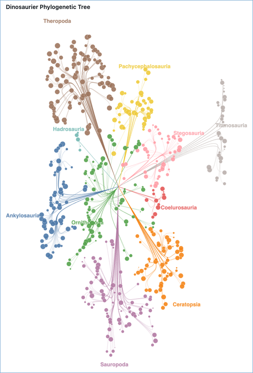
Custom visualizations can render specialized chart types that go beyond the built-in options. The following phylogenetic tree uses a force-directed layout to group related records around shared group and family centers:
To build a chart step by step, see Example visualizations. To reference the specifications for other chart types, see More chart specifications.
Create a custom visualization
To create a custom visualization:
- Select a dataset.
- In the visualization configuration pane, select Custom Viz under the Advanced visualization section.
- In the Fields section, add the fields you want to use. Each field has a unique Name. Reference fields in your Vega-Lite specification using these names.
- Enter your Vega-Lite JSON specification in the Vega-Lite specification editor.
Reference dataset columns
Reference columns in a Vega-Lite specification in one of the following ways:
-
Use
"field": "{columnName}". The following example assigns thexFieldcolumn to the x-axis:JSON"encoding": {
"x": { "field": "xField", "type": "quantitative" }
} -
In expressions, use
datum["{columnName}"]ordatum.{columnName}. The following example defines a newxcolumn from therandanglecolumns:JSON{ "calculate": "datum.r * cos(datum.angle)", "as": "x" }
For more information, see datum in the Vega expressions documentation.
Inherit the dashboard theme
Custom visualizations automatically adapt to the dashboard's theme, including light and dark mode. The following chart elements inherit theme values without any changes to your specification:
- Axis, legend, title, and header fonts match the dashboard's configured fonts.
- Axis grid lines match the dashboard's gridline color for the active mode.
- The chart background is transparent over the widget's themed background.
Settings you define in your specification's config block take precedence over the inherited defaults.
Reference theme values in expressions
To style marks with theme-aware values, reference the following signals inside a Vega-Lite expression ({ "expr": "..." }):
Signal | Description |
|---|---|
| Pre-resolved color tokens for the active mode. Use these for common values such as |
| The active color mode, either |
| The full theme configured by the dashboard owner, including fonts ( |
The colors and dashboardTheme signals are independent. The colors signal provides convenience tokens resolved for the active mode, while dashboardTheme exposes the complete owner-configured theme. Use colors first, and use dashboardTheme for fonts, the full palette, or any value colors doesn't provide.
The following examples demonstrate how to reference theme values:
-
Use the dashboard's body font for a text mark:
JSON{ "expr": "dashboardTheme.resolvedFontSettings.fieldValue.fontFamily" } -
Use the dashboard's title color for the active mode:
JSON{ "expr": "dashboardTheme.resolvedFontSettings.fieldTitle.fontColor[mode]" } -
Use a color from the dashboard's categorical palette:
JSON{ "expr": "dashboardTheme.visualizationColors[0]" }
The colors tokens are already resolved for the active mode. Skip the [mode] index and use colors.markHighlightColor, not colors.markHighlightColor[mode]. Fields under dashboardTheme that have per-mode variants, such as dashboardTheme.gridLineColor[mode], require the [mode] index.
Filter other widgets on selection
A custom visualization can act as a cross-filter source: when a user clicks a mark, the selection filters the other widgets on the dashboard. To enable this, add a point selection parameter with the reserved name databricks_mark_selection. The renderer detects this name and connects the selection to the dashboard's cross-filter state.
"params": [
  {
    "name": "databricks_mark_selection",
    "select": { "type": "point", "fields": ["categoryName"] }
  }
]
The following requirements apply:
- The parameter
namemust be exactlydatabricks_mark_selection. Any other name is treated as a regular parameter and does not drive cross-filtering. select.typemust bepoint. Interval (brush) selections are not supported as cross-filter sources.select.fieldsmust list the field names defined in the Fields section of the widget configuration, not the raw column names.- List only dimension (grouping) fields in
select.fields. Aggregated measures, such asSUM(...)orAVG(...), cannot drive a cross-filter. - To select on multiple fields, list them together:
"fields": ["categoryName", "regionName"].
Highlight selected marks
To highlight selected marks, use stroke and strokeWidth conditions on a fill-based mark (such as bar, arc, or rect) and keep the color encoding bound to your field. Use { "expr": "colors.markHighlightColor" } for the stroke so the highlight stays legible in both light and dark modes.
The following example filters the rest of the dashboard by categoryName when a bar is clicked. Selected bars get a themed stroke, and unselected bars dim while keeping their color encoding.
JSON specification
{
  "$schema": "https://vega.github.io/schema/vega-lite/v6.json",
  "data": { "name": "databricks_query" },
  "width": "container",
  "height": "container",
  "config": { "autosize": { "type": "fit", "contains": "padding" } },
  "params": [
    {
      "name": "databricks_mark_selection",
      "select": { "type": "point", "fields": ["categoryName"] }
    }
  ],
  "mark": { "type": "bar", "stroke": null },
  "encoding": {
    "x": { "field": "categoryName", "type": "nominal" },
    "y": { "field": "salesValue", "type": "quantitative" },
    "color": { "field": "categoryName", "type": "nominal" },
    "fillOpacity": {
      "condition": { "param": "databricks_mark_selection", "value": 1 },
      "value": 0.3
    },
    "stroke": {
      "condition": {
        "param": "databricks_mark_selection",
        "empty": false,
        "value": { "expr": "colors.markHighlightColor" }
      },
      "value": null
    },
    "strokeWidth": {
      "condition": { "param": "databricks_mark_selection", "empty": false, "value": 2 },
      "value": 0
    }
  }
}
Resize a chart automatically
To make a chart resize to fit its container, add the following settings at the top level of your specification:
"width": "container",
"height": "container",
"config": {
  "autosize": {
    "type": "fit",
    "contains": "padding"
  }
}
Example visualizations
The following examples walk through building a custom visualization step by step, from a simple layered chart to a more advanced phylogenetic tree.
Layered chart with a rolling mean
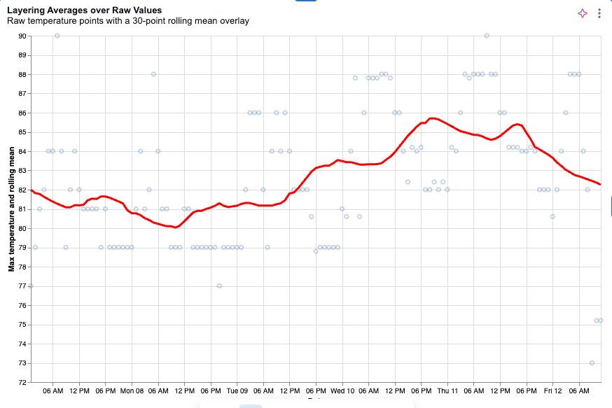
This example creates a layered chart that plots raw temperature data points with a rolling mean line overlay, using weather data from the Databricks sample datasets.
-
Create a dataset with the following query:
SQLSELECT date, temperature AS temp_max
FROM samples.accuweather.historical_hourly_imperial
WHERE city_name = 'singapore'
ORDER BY date; -
In the visualization configuration pane, under Advanced, select Custom Viz.
-
Select the dataset you created in the previous step.
-
In the Fields section, add a field for the date column and set its Name to
date. -
Add a field for the temperature column and set its Name to
temp_max. -
Copy the following specification into the Vega-Lite specification editor. If the x-axis is clipped, see Resize a chart automatically.
JSON specification
JSON{
"$schema": "https://vega.github.io/schema/vega-lite/v5.json",
"width": "container",
"height": "container",
"config": {
"autosize": { "type": "fit", "contains": "padding" }
},
"data": { "name": "databricks_query" },
"transform": [
{
"window": [{ "field": "temp_max", "op": "mean", "as": "rolling_mean" }],
"frame": [-15, 15]
}
],
"encoding": {
"x": { "field": "date", "type": "temporal", "title": "Date" },
"y": {
"type": "quantitative",
"scale": { "zero": false },
"axis": { "title": "Max temperature and rolling mean" }
}
},
"layer": [
{
"mark": { "type": "point", "opacity": 0.3 },
"encoding": { "y": { "field": "temp_max", "title": "Max temperature" } }
},
{
"mark": { "type": "line", "color": "red", "size": 3 },
"encoding": { "y": { "field": "rolling_mean", "title": "Rolling mean of max temperature" } }
}
]
}
Phylogenetic tree
This example uses a small set of sample data to build the phylogenetic tree shown at the top of this page. Vega-Lite plots points at the coordinates you provide, but it doesn't calculate node positions for a network diagram itself. That calculation happens in the query before the data reaches the chart, where the query precomputes each point's x and y coordinates. The query emits three record types that the specification renders as separate layers: path rows draw the curved branches, node rows draw the leaf circles, and label rows position the group labels.
-
Download the sample data. Each row represents a fossil find, with
dig_longitudeanddig_latitudegiving its dig-site coordinates. -
Click
 Dashboards in the sidebar.
 -
Click Create dashboard.
-
Click the Data tab.
-
Click Add data, then click Upload data.
-
Drop the downloaded file into the Create or modify table from file upload pane.
-
Choose the Catalog and Schema where you want to store the table, then enter a table name.
-
Click Create table. The full table is automatically added as a dataset.
-
Click Add SQL dataset and paste in the query. In the query's
FROMclause, replace the catalog, schema, and table names with the ones you used when you created the table. -
Create the custom visualization, following the steps in Create a custom visualization. In the Fields section, add the following fields, using each field name as its Name:
record_type,x,y,fossil_tag,point_order,suborder,roar_score,clade_label,genus_symbol,family_taxon, andlabel_text. Use the specification as your Vega-Lite JSON.
SQL query
WITH base AS (
  SELECT
    fossil_tag,
    genus_symbol,
    clade_label,
    suborder,
    family_taxon,
    dig_longitude,
    dig_latitude,
    roar_score
  FROM
    `my_catalog`.`default`.`dino_table`
),
root_pt AS (
  SELECT
    AVG(dig_longitude) AS rx,
    AVG(dig_latitude) AS ry
  FROM
    base
),
group_pts AS (
  SELECT
    suborder,
    AVG(dig_longitude) AS gx,
    AVG(dig_latitude) AS gy
  FROM
    base
  GROUP BY
    suborder
),
family_pts AS (
  SELECT
    suborder,
    family_taxon,
    AVG(dig_longitude) AS fx,
    AVG(dig_latitude) AS fy
  FROM
    base
  GROUP BY
    suborder,
    family_taxon
),
ctx AS (
  SELECT
    b.fossil_tag,
    b.suborder,
    b.family_taxon,
    b.clade_label,
    b.genus_symbol,
    b.dig_longitude,
    b.dig_latitude,
    b.roar_score,
    r.rx,
    r.ry,
    g.gx,
    g.gy,
    f.fx,
    f.fy
  FROM
    base b
      CROSS JOIN root_pt r
      JOIN group_pts g
        ON b.suborder = g.suborder
      JOIN family_pts f
        ON b.suborder = f.suborder
        AND b.family_taxon = f.family_taxon
),
waypoints AS (
  SELECT
    fossil_tag,
    suborder,
    family_taxon,
    clade_label,
    genus_symbol,
    roar_score,
    0 AS point_order,
    rx AS x,
    ry AS y
  FROM
    ctx
  UNION ALL
  SELECT
    fossil_tag,
    suborder,
    family_taxon,
    clade_label,
    genus_symbol,
    roar_score,
    1,
    rx + 0.30 * (gx - rx),
    ry + 0.30 * (gy - ry)
  FROM
    ctx
  UNION ALL
  SELECT
    fossil_tag,
    suborder,
    family_taxon,
    clade_label,
    genus_symbol,
    roar_score,
    2,
    gx + 0.15 * (fx - gx),
    gy + 0.15 * (fy - gy)
  FROM
    ctx
  UNION ALL
  SELECT
    fossil_tag,
    suborder,
    family_taxon,
    clade_label,
    genus_symbol,
    roar_score,
    3,
    gx + 0.50 * (fx - gx) + 0.03 * (dig_longitude - fx),
    gy + 0.50 * (fy - gy) + 0.03 * (dig_latitude - fy)
  FROM
    ctx
  UNION ALL
  SELECT
    fossil_tag,
    suborder,
    family_taxon,
    clade_label,
    genus_symbol,
    roar_score,
    4,
    fx + 0.15 * (dig_longitude - fx),
    fy + 0.15 * (dig_latitude - fy)
  FROM
    ctx
  UNION ALL
  SELECT
    fossil_tag,
    suborder,
    family_taxon,
    clade_label,
    genus_symbol,
    roar_score,
    5,
    fx + 0.65 * (dig_longitude - fx),
    fy + 0.65 * (dig_latitude - fy)
  FROM
    ctx
  UNION ALL
  SELECT
    fossil_tag,
    suborder,
    family_taxon,
    clade_label,
    genus_symbol,
    roar_score,
    6,
    dig_longitude,
    dig_latitude
  FROM
    ctx
)
SELECT
  fossil_tag,
  suborder,
  point_order,
  x,
  y,
  family_taxon,
  clade_label,
  genus_symbol,
  roar_score,
  'path' AS record_type,
  CAST(NULL AS STRING) AS label_text
FROM
  waypoints
UNION ALL
SELECT
  fossil_tag,
  suborder,
  99 AS point_order,
  dig_longitude AS x,
  dig_latitude AS y,
  family_taxon,
  clade_label,
  genus_symbol,
  roar_score,
  'node' AS record_type,
  CAST(NULL AS STRING) AS label_text
FROM
  base
UNION ALL
SELECT
  g.suborder AS fossil_tag,
  g.suborder AS suborder,
  100 AS point_order,
  g.gx
    + (g.gx - r.rx)
      * CASE LOWER(g.suborder)
        WHEN 'titanosauria' THEN 0.10
        WHEN 'hadrosauria' THEN 0.25
        WHEN 'ornithopoda' THEN 1.30
        WHEN 'stegosauria' THEN 0.73
        ELSE 0.55
      END AS x,
  g.gy
    + (g.gy - r.ry)
      * CASE LOWER(g.suborder)
        WHEN 'titanosauria' THEN 0.10
        WHEN 'hadrosauria' THEN 0.25
        WHEN 'ornithopoda' THEN 1.30
        WHEN 'stegosauria' THEN 0.73
        ELSE 0.55
      END AS y,
  CAST(NULL AS STRING) AS family_taxon,
  CAST(NULL AS STRING) AS clade_label,
  CAST(NULL AS STRING) AS genus_symbol,
  CAST(NULL AS DOUBLE) AS roar_score,
  'label' AS record_type,
  g.suborder AS label_text
FROM
  group_pts g CROSS JOIN root_pt r
JSON specification
{
  "$schema": "https://vega.github.io/schema/vega-lite/v5.json",
  "data": { "name": "databricks_query" },
  "width": "container",
  "height": "container",
  "background": "white",
  "config": {
    "autosize": { "type": "fit", "contains": "padding" },
    "view": { "stroke": null }
  },
  "layer": [
    {
      "transform": [{ "filter": "datum.record_type === 'path'" }],
      "mark": {
        "type": "line",
        "interpolate": "basis",
        "strokeCap": "round",
        "strokeJoin": "round"
      },
      "encoding": {
        "x": {
          "field": "x",
          "type": "quantitative",
          "axis": null,
          "scale": { "zero": false, "nice": false }
        },
        "y": {
          "field": "y",
          "type": "quantitative",
          "axis": null,
          "scale": { "zero": false, "nice": false }
        },
        "detail": { "field": "fossil_tag", "type": "nominal" },
        "order": { "field": "point_order", "type": "quantitative" },
        "color": {
          "field": "suborder",
          "type": "nominal",
          "scale": { "scheme": "tableau10" },
          "legend": null
        },
        "opacity": { "value": 0.3 },
        "strokeWidth": { "value": 0.8 }
      }
    },
    {
      "transform": [{ "filter": "datum.record_type === 'node'" }],
      "mark": {
        "type": "circle",
        "opacity": 0.9,
        "stroke": "white",
        "strokeWidth": 0.3
      },
      "encoding": {
        "x": {
          "field": "x",
          "type": "quantitative",
          "axis": null,
          "scale": { "zero": false, "nice": false }
        },
        "y": {
          "field": "y",
          "type": "quantitative",
          "axis": null,
          "scale": { "zero": false, "nice": false }
        },
        "color": {
          "field": "suborder",
          "type": "nominal",
          "scale": { "scheme": "tableau10" },
          "legend": { "title": "Suborder", "orient": "right" }
        },
        "size": {
          "field": "roar_score",
          "type": "quantitative",
          "scale": { "domain": [0, 100], "range": [4, 150] },
          "legend": null
        },
        "tooltip": [
          { "field": "clade_label", "title": "Clade" },
          { "field": "genus_symbol", "title": "Symbol" },
          { "field": "suborder", "title": "Suborder" },
          { "field": "family_taxon", "title": "Family" },
          { "field": "roar_score", "title": "Roar Score", "format": ".1f" }
        ]
      }
    },
    {
      "transform": [{ "filter": "datum.record_type === 'label'" }],
      "mark": {
        "type": "text",
        "fontSize": 12,
        "fontWeight": "bold",
        "opacity": 0.85
      },
      "encoding": {
        "x": {
          "field": "x",
          "type": "quantitative",
          "axis": null,
          "scale": { "zero": false, "nice": false }
        },
        "y": {
          "field": "y",
          "type": "quantitative",
          "axis": null,
          "scale": { "zero": false, "nice": false }
        },
        "text": { "field": "label_text", "type": "nominal" },
        "color": {
          "field": "suborder",
          "type": "nominal",
          "scale": { "scheme": "tableau10" },
          "legend": null
        }
      }
    }
  ]
}
More chart specifications
The following specifications show charts that aren't available as built-in visualization types. For more examples, see the Vega-Lite example galleries.
Bullet chart
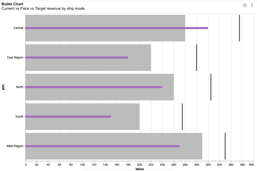
Define categoryField, currentField, paceField, and targetField in the Fields section.
JSON specification
{
  "$schema": "https://vega.github.io/schema/vega-lite/v5.json",
  "width": "container",
  "height": "container",
  "data": { "name": "databricks_query" },
  "config": {
    "autosize": { "type": "fit", "contains": "padding" }
  },
  "transform": [
    {
      "fold": ["targetField", "paceField", "currentField"],
      "as": ["measure_name", "measure_value"]
    },
    {
      "calculate": "toNumber(datum.measure_value)",
      "as": "measure_value"
    },
    {
      "calculate": "{ \"targetField\": \"Target\", \"paceField\": \"Pace\", \"currentField\": \"Current\" }[datum.measure_name]",
      "as": "measure_label"
    },
    {
      "calculate": "indexof([\"Target\", \"Pace\", \"Current\"], datum.measure_label)",
      "as": "measure_order"
    }
  ],
  "layer": [
    {
      "mark": "bar",
      "params": [
        {
          "name": "legend_click",
          "select": { "type": "point", "fields": ["measure_label"] },
          "bind": "legend"
        }
      ],
      "encoding": {
        "color": { "field": "measure_label" },
        "opacity": { "value": 0 }
      }
    },
    {
      "transform": [{ "filter": { "param": "legend_click" } }],
      "layer": [
        {
          "layer": [
            {
              "mark": { "type": "bar", "tooltip": true },
              "encoding": { "color": { "field": "measure_label", "legend": null } },
              "transform": [{ "filter": { "field": "measure_label", "oneOf": ["Pace"] } }]
            },
            {
              "mark": { "type": "bar", "height": 7, "tooltip": true },
              "encoding": { "color": { "field": "measure_label", "legend": null } },
              "transform": [{ "filter": { "field": "measure_label", "oneOf": ["Current"] } }]
            },
            {
              "mark": { "type": "tick", "tooltip": true, "thickness": 3 },
              "encoding": { "color": { "field": "measure_label", "legend": null } },
              "transform": [{ "filter": { "field": "measure_label", "oneOf": ["Target"] } }]
            }
          ],
          "encoding": {
            "x": {
              "field": "measure_value",
              "type": "quantitative",
              "stack": null,
              "title": "Value",
              "axis": { "orient": "bottom" }
            },
            "color": {
              "scale": {
                "domain": ["Target", "Pace", "Current"],
                "range": ["#000000", "#bcbcbc", "#A66BBF"]
              }
            },
            "order": {
              "field": "measure_order",
              "type": "quantitative",
              "sort": "descending"
            }
          }
        }
      ],
      "encoding": {
        "y": {
          "field": "categoryField",
          "type": "ordinal",
          "title": "Category",
          "axis": { "labelOverlap": true }
        },
        "tooltip": [
          { "field": "categoryField", "type": "nominal", "title": "Category" },
          { "field": "currentField", "type": "quantitative", "title": "Current" },
          { "field": "paceField", "type": "quantitative", "title": "Pace" },
          { "field": "targetField", "type": "quantitative", "title": "Target" }
        ]
      }
    }
  ]
}
Gauge
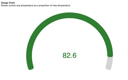
Define $valueField and $totalField in the Fields section.
JSON specification
{
  "$schema": "https://vega.github.io/schema/vega-lite/v6.json",
  "width": "container",
  "height": "container",
  "data": { "name": "databricks_query" },
  "config": {
    "concat": { "spacing": 0 },
    "autosize": { "type": "fit", "contains": "padding" }
  },
  "params": [
    { "name": "ring_max", "expr": "min(width, height) / 2 - 16" },
    { "name": "ring_width", "expr": "max(12, (min(width, height) / 2) * 0.12)" },
    { "name": "ring_gap", "expr": "max(4, (min(width, height) / 2) * 0.03)" },
    { "name": "label_color", "value": "#000000" },
    { "name": "ring_background_opacity", "value": 0.3 },
    { "name": "ring0_percent", "value": 100 },
    { "name": "ring0_outer", "expr": "ring_max + 2" },
    { "name": "ring0_inner", "expr": "ring_max + 1" },
    { "name": "ring1_outer", "expr": "ring0_inner - ring_gap" },
    { "name": "ring1_inner", "expr": "ring1_outer - ring_width" },
    { "name": "ring1_middle", "expr": "(ring1_outer + ring1_inner) / 2" },
    { "name": "arc_size", "expr": "220" }
  ],
  "transform": [
    { "as": "ratio", "calculate": "datum['$valueField'] / datum['$totalField']" },
    { "as": "_arc_start_degrees", "calculate": "360 - ( arc_size / 2 )" },
    { "as": "_arc_end_degrees", "calculate": "0 + ( arc_size / 2 )" },
    { "as": "_arc_start_radians", "calculate": "2 * 3.14 * ( datum['_arc_start_degrees'] - 360 ) / 360" },
    { "as": "_arc_end_radians", "calculate": "2 * 3.14 * datum['_arc_end_degrees'] / 360" },
    { "as": "_arc_total_radians", "calculate": "datum['_arc_end_radians'] - datum['_arc_start_radians']" },
    { "as": "_ring_start_radians", "calculate": "datum['_arc_start_radians']" },
    {
      "as": "_ring_end_radians",
      "calculate": "datum['_arc_start_radians'] + ( datum['_arc_total_radians'] * datum['ratio'] )"
    }
  ],
  "layer": [
    {
      "mark": {
        "type": "arc",
        "color": "lightgrey",
        "theta": { "expr": "datum['_arc_start_radians']" },
        "radius": { "expr": "ring1_outer" },
        "theta2": { "expr": "datum['_arc_end_radians']" },
        "radius2": { "expr": "ring1_inner" },
        "cornerRadius": 10
      }
    },
    {
      "name": "RING",
      "mark": {
        "type": "arc",
        "theta": { "expr": "datum['_ring_start_radians']" },
        "radius": { "expr": "ring1_outer" },
        "theta2": { "expr": "datum['_ring_end_radians']" },
        "radius2": { "expr": "ring1_inner" },
        "cornerRadius": 10
      },
      "encoding": {
        "color": {
          "value": "#307E31",
          "condition": [
            { "test": "datum['ratio'] < 0.33", "value": "#880808" },
            { "test": "datum['ratio'] < 0.66", "value": "#E49B0F" }
          ]
        }
      }
    },
    {
      "mark": { "type": "text", "fontSize": 40 },
      "encoding": {
        "text": { "field": "$valueField" },
        "color": {
          "value": "#307E31",
          "condition": [
            { "test": "datum['ratio'] < 0.33", "value": "#880808" },
            { "test": "datum['ratio'] < 0.66", "value": "#E49B0F" }
          ]
        }
      }
    }
  ]
}
Radar chart
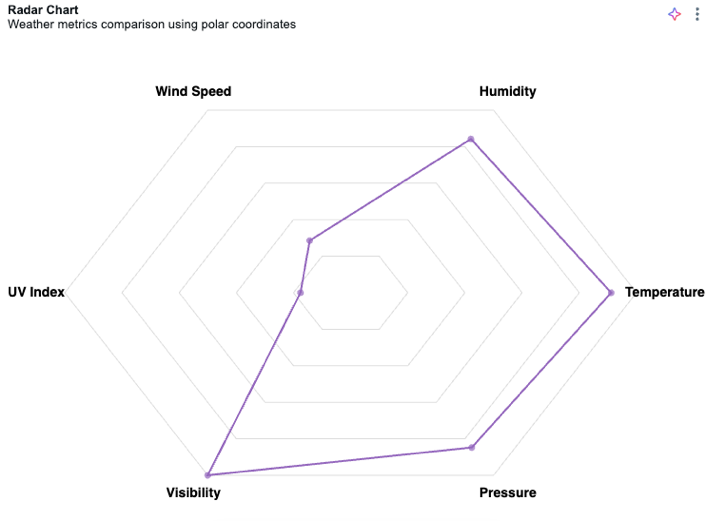
Define $key and $value in the Fields section.
JSON specification
{
  "$schema": "https://vega.github.io/schema/vega-lite/v5.json",
  "width": "container",
  "height": "container",
  "config": {
    "autosize": { "type": "fit", "contains": "padding" }
  },
  "data": { "name": "databricks_query" },
  "transform": [
    { "window": [{ "op": "row_number", "as": "category" }] },
    { "calculate": "datum.category - 1", "as": "category" },
    {
      "joinaggregate": [
        { "op": "count", "as": "numCategories" },
        { "op": "max", "field": "$value", "as": "maxValue" }
      ]
    },
    { "calculate": "2 * PI * datum.category / datum.numCategories", "as": "angle" },
    { "calculate": "100 * datum['$value'] / datum.maxValue", "as": "r" },
    { "calculate": "datum.r * cos(datum.angle)", "as": "x" },
    { "calculate": "datum.r * sin(datum.angle)", "as": "y" },
    { "calculate": "110 * cos(datum.angle)", "as": "label_x" },
    { "calculate": "110 * sin(datum.angle)", "as": "label_y" }
  ],
  "layer": [
    {
      "transform": [
        { "joinaggregate": [{ "op": "count", "as": "numCategories" }] },
        { "aggregate": [{ "op": "max", "field": "numCategories", "as": "numCategories" }] },
        { "calculate": "[0,1,2,3,4,5,6,7,8,9,10,11,12,13,14,15,16,17,18,19,20]", "as": "cats" },
        { "flatten": ["cats"], "as": ["cat"] },
        { "filter": "datum.cat <= datum.numCategories" },
        { "calculate": "2 * PI * datum.cat / datum.numCategories", "as": "angle" },
        { "calculate": "100 * cos(datum.angle)", "as": "x" },
        { "calculate": "100 * sin(datum.angle)", "as": "y" }
      ],
      "mark": { "type": "line", "color": "#ddd", "strokeWidth": 1 },
      "encoding": {
        "x": { "field": "x", "type": "quantitative", "scale": { "domain": [-120, 120] }, "axis": null },
        "y": { "field": "y", "type": "quantitative", "scale": { "domain": [-120, 120] }, "axis": null },
        "order": { "field": "cat" }
      }
    },
    {
      "transform": [
        { "joinaggregate": [{ "op": "count", "as": "numCategories" }] },
        { "aggregate": [{ "op": "max", "field": "numCategories", "as": "numCategories" }] },
        { "calculate": "[20,40,60,80,100]", "as": "levels" },
        { "flatten": ["levels"], "as": ["level"] },
        { "calculate": "[0,1,2,3,4,5,6,7,8,9,10,11,12,13,14,15,16,17,18,19,20]", "as": "cats" },
        { "flatten": ["cats"], "as": ["cat"] },
        { "filter": "datum.cat <= datum.numCategories" },
        { "calculate": "2 * PI * datum.cat / datum.numCategories", "as": "angle" },
        { "calculate": "datum.level", "as": "r" },
        { "calculate": "datum.r * cos(datum.angle)", "as": "x" },
        { "calculate": "datum.r * sin(datum.angle)", "as": "y" }
      ],
      "mark": { "type": "line", "color": "#ddd", "strokeWidth": 1 },
      "encoding": {
        "x": { "field": "x", "type": "quantitative" },
        "y": { "field": "y", "type": "quantitative" },
        "detail": { "field": "level" },
        "order": { "field": "cat" }
      }
    },
    {
      "mark": { "type": "line", "color": "#9467bd", "strokeWidth": 2, "interpolate": "linear-closed" },
      "encoding": {
        "x": { "field": "x", "type": "quantitative" },
        "y": { "field": "y", "type": "quantitative" },
        "order": { "field": "category" }
      }
    },
    {
      "mark": { "type": "point", "filled": true, "size": 50, "color": "#9467bd" },
      "encoding": {
        "x": { "field": "x", "type": "quantitative" },
        "y": { "field": "y", "type": "quantitative" }
      }
    },
    {
      "mark": { "type": "text", "fontSize": 14, "fontWeight": "bold" },
      "encoding": {
        "x": { "field": "label_x", "type": "quantitative" },
        "y": { "field": "label_y", "type": "quantitative" },
        "text": { "field": "$key", "type": "nominal" }
      }
    }
  ],
  "view": { "stroke": null }
}
Radial chart
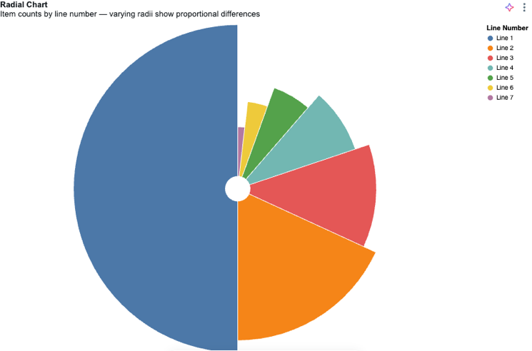
Define $valueField and $colorField in the Fields section.
JSON specification
{
  "$schema": "https://vega.github.io/schema/vega-lite/v6.json",
  "width": "container",
  "height": "container",
  "config": {
    "autosize": { "type": "fit", "contains": "padding" }
  },
  "data": { "name": "databricks_query" },
  "transform": [
    {
      "aggregate": [{ "op": "sum", "field": "$valueField", "as": "total" }],
      "groupby": ["$colorField"]
    },
    {
      "window": [{ "op": "rank", "as": "rank" }],
      "sort": [{ "field": "total", "order": "descending" }]
    }
  ],
  "layer": [
    {
      "mark": { "type": "arc", "innerRadius": 20, "stroke": "#fff" }
    }
  ],
  "encoding": {
    "theta": {
      "field": "total",
      "type": "quantitative",
      "scale": { "type": "sqrt" },
      "stack": true,
      "sort": "descending"
    },
    "radius": { "field": "total", "scale": { "type": "sqrt", "zero": true } },
    "color": {
      "field": "$colorField",
      "type": "nominal",
      "title": "Sub-Category",
      "sort": { "field": "total", "order": "descending" },
      "legend": { "orient": "right" }
    },
    "tooltip": [
      { "field": "$colorField", "type": "nominal", "title": "Sub-Category" },
      { "field": "total", "type": "quantitative", "title": "Sales" }
    ]
  },
  "view": { "stroke": null }
}
Sunburst chart
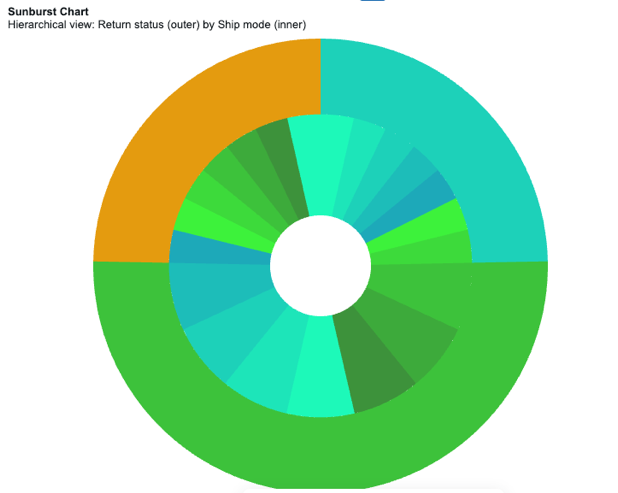
Define outerGroupField, innerGroupField, and sizeField in the Fields section.
JSON specification
{
  "$schema": "https://vega.github.io/schema/vega-lite/v5.json",
  "width": "container",
  "height": "container",
  "data": { "name": "databricks_query" },
  "config": {
    "autosize": { "type": "fit", "contains": "padding" }
  },
  "transform": [
    { "calculate": "datum['outerGroupField']", "as": "OUTSIDE" },
    { "calculate": "datum['innerGroupField']", "as": "INSIDE" },
    { "calculate": "datum.OUTSIDE + '-' + datum.INSIDE", "as": "OUT_IN" },
    { "calculate": "toNumber(datum['sizeField'])", "as": "SIZE" }
  ],
  "resolve": {
    "scale": { "color": "independent" },
    "legend": { "color": "independent" }
  },
  "layer": [
    {
      "mark": {
        "type": "arc",
        "tooltip": true,
        "innerRadius": { "expr": "min(width, height)/9" },
        "outerRadius": { "expr": "min(width, height)/3" }
      },
      "encoding": {
        "theta": { "field": "SIZE", "type": "quantitative", "stack": true },
        "color": {
          "field": "OUT_IN",
          "type": "ordinal",
          "sort": "ascending",
          "title": "Inner Grouping",
          "scale": {
            "range": [
              "#1DF9B9",
              "#1DE5B9",
              "#1DD1B9",
              "#1DBDB9",
              "#1DA9B9",
              "#3DF23B",
              "#3DDA3B",
              "#3DC23B",
              "#3DAA3B",
              "#3D923B"
            ]
          }
        },
        "order": { "field": "OUT_IN", "sort": "ascending" },
        "tooltip": [
          { "field": "OUTSIDE", "type": "nominal", "title": "Outer Grouping" },
          { "field": "INSIDE", "type": "nominal", "title": "Inner Grouping" },
          { "field": "SIZE", "type": "quantitative", "title": "Count" }
        ]
      }
    },
    {
      "transform": [
        {
          "aggregate": [{ "op": "sum", "field": "SIZE", "as": "total_users" }],
          "groupby": ["OUTSIDE"]
        }
      ],
      "mark": {
        "type": "arc",
        "tooltip": true,
        "innerRadius": { "expr": "min(width, height)/3" }
      },
      "encoding": {
        "theta": {
          "field": "total_users",
          "type": "quantitative",
          "stack": true,
          "sort": "ascending",
          "title": "Users Count"
        },
        "color": {
          "field": "OUTSIDE",
          "type": "ordinal",
          "sort": "ascending",
          "title": "Outer Grouping",
          "scale": { "range": ["#1DD1B9", "#3DC23B"] }
        },
        "order": { "field": "OUTSIDE", "sort": "ascending" },
        "tooltip": [
          { "field": "OUTSIDE", "type": "nominal", "title": "Outer Grouping" },
          { "field": "total_users", "type": "quantitative", "title": "Count" }
        ]
      }
    }
  ]
}
Limitations
- Treemap charts aren't supported. Vega-Lite doesn't support treemaps.
- Image marks support only inline base64
data:image URLs (for example,data:image/png;base64,...) of 37 KB or less, in PNG, JPEG, or WebP format. Remote image URLs (https:orhttp:), relative URLs, SVG images, and field- or expression-driven image URLs aren't supported.