Transform data with pipelines
You declare transformations in pipelines to specify how records are processed through query logic, using common patterns like stream-static joins, incremental aggregations, and mixing streaming tables and materialized views.
You can define a dataset against any query that returns a DataFrame. You can use Apache Spark built-in operations, UDFs, custom logic, and MLflow models as transformations in Lakeflow Spark Declarative Pipelines. After data has been ingested into your pipeline, you can define new datasets against upstream sources to create new streaming tables, materialized views, and views.
For guidance on choosing between views, materialized views, and streaming tables, see What are pipelines?. To learn how to effectively perform stateful processing in a pipeline, see Optimize stateful processing with watermarks.
Exclude tables from the target schema
If you must calculate intermediate tables not intended for external consumption, you can prevent them from being published to a schema using the PRIVATE keyword. Private tables still store and process data according to Lakeflow Spark Declarative Pipelines semantics but should not be accessed outside the current pipeline. A private table persists for the lifetime of the pipeline that creates it. Use the following syntax to declare private tables:
- SQL
- Python
CREATE PRIVATE STREAMING TABLE private_table
AS SELECT ... ;
@dp.table(
  private=True)
def private_table():
  return ("...")
Combine streaming tables and materialized views in a single pipeline
Streaming tables inherit the processing guarantees of Apache Spark Structured Streaming and are configured to process queries from append-only data sources, where new rows are always inserted into the source table rather than modified.
Although, by default, streaming tables require append-only data sources, when a streaming source is another streaming table that requires updates or deletes, you can override this behavior with the skipChangeCommits flag
A common streaming pattern involves ingesting source data to create the initial datasets in a pipeline. These initial datasets are commonly called bronze tables and often perform simple transformations.
By contrast, the final tables in a pipeline, commonly called gold tables, often require complicated aggregations or reading from targets of an AUTO CDC ... INTO operation. Because these operations inherently create updates rather than appends, they are not supported as inputs to streaming tables. These transformations are better suited for materialized views.
By mixing streaming tables and materialized views into a single pipeline, you can simplify your pipeline, avoid costly re-ingestion or re-processing of raw data, and have the full power of SQL to compute complex aggregations over an efficiently encoded and filtered dataset. The following example illustrates this type of mixed processing:
These examples use Auto Loader to load files from cloud storage. To load files with Auto Loader in a Unity Catalog enabled pipeline, you must use external locations. To learn more about using Unity Catalog with pipelines, see Use Unity Catalog with pipelines.
- Python
- SQL
@dp.table
def streaming_bronze():
  return (
    # Since this is a streaming source, this table is incremental.
    spark.readStream.format("cloudFiles")
      .option("cloudFiles.format", "json")
      .load("s3://path/to/raw/data")
  )

@dp.table
def streaming_silver():
  # Since we read the bronze table as a stream, this silver table is also
  # updated incrementally.
  return spark.readStream.table("streaming_bronze").where(...)

@dp.materialized_view
def live_gold():
  # This table will be recomputed completely by reading the whole silver table
  # when it is updated.
  return spark.read.table("streaming_silver").groupBy("user_id").count()
CREATE OR REFRESH STREAMING TABLE streaming_bronze
AS SELECT * FROM STREAM read_files(
  "s3://path/to/raw/data",
  format => "json"
)

CREATE OR REFRESH STREAMING TABLE streaming_silver
AS SELECT * FROM STREAM(streaming_bronze) WHERE...

CREATE OR REFRESH MATERIALIZED VIEW mv_gold
AS SELECT count(*) FROM streaming_silver GROUP BY user_id
Learn more about using Auto Loader to incrementally ingest JSON files from S3.
Stream-static joins
Stream-static joins are a good choice when denormalizing a continuous stream of append-only data with a primarily static dimension table.
With each pipeline update, new records from the stream are joined with the most current snapshot of the static table. If records are added or updated in the static table after corresponding data from the streaming table has been processed, the resultant records are not recalculated unless a full refresh is performed.
In pipelines configured for triggered execution, the static table returns results as of the time the update started. In pipelines configured for continuous execution, the most recent version of the static table is queried each time the table processes an update.
The following is an example of a stream-static join:
- Python
- SQL
@dp.table
def customer_sales():
  return spark.readStream.table("sales").join(spark.read.table("customers"), ["customer_id"], "left")
CREATE OR REFRESH STREAMING TABLE customer_sales
AS SELECT * FROM STREAM(sales)
  INNER JOIN LEFT customers USING (customer_id)
Calculate aggregates efficiently
You can use streaming tables to incrementally calculate simple distributive aggregates like count, min, max, or sum, and algebraic aggregates like average or standard deviation. Databricks recommends incremental aggregation for queries with a limited number of groups, such as a query with a GROUP BY country clause. Only new input data is read with each update.
To learn more about writing Lakeflow Spark Declarative Pipelines queries that perform incremental aggregations, see Perform windowed aggregations with watermarks.
Use MLflow models in Lakeflow Spark Declarative Pipelines
To use MLflow models in a Unity Catalog-enabled pipeline, your pipeline must be configured to use the preview channel. To use the current channel, you must configure your pipeline to publish to the Hive metastore.
You can use MLflow-trained models in pipelines. MLflow models are treated as transformations in Databricks, meaning they act upon a Spark DataFrame input and return results as a Spark DataFrame. Because Lakeflow Spark Declarative Pipelines defines datasets against DataFrames, you can convert Apache Spark workloads that use MLflow into pipelines with just a few lines of code. For more on MLflow, see MLflow on Databricks.
If you already have a Python script calling an MLflow model, you can adapt this code to a pipeline by using the @dp.table or @dp.materialized_view decorator and ensuring functions are defined to return transformation results. Lakeflow Spark Declarative Pipelines does not install MLflow by default, so confirm that you have installed the MLFlow libraries with %pip install mlflow and have imported mlflow and dp at the top of your source. For an introduction to pipeline syntax, see Develop pipeline code with Python.
To use MLflow models in pipelines, complete the following steps:
- Obtain the run ID and model name of the MLflow model. The run ID and model name are used to construct the URI of the MLflow model.
- Use the URI to define a Spark UDF to load the MLflow model.
- Call the UDF in your table definitions to use the MLflow model.
The following example shows the basic syntax for this pattern:
%pip install mlflow==2.20.2

from pyspark import pipelines as dp
import mlflow

run_id= "<mlflow-run-id>"
model_name = "<the-model-name-in-run>"
model_uri = f"runs:/{run_id}/{model_name}"
loaded_model_udf = mlflow.pyfunc.spark_udf(spark, model_uri=model_uri)

@dp.materialized_view
def model_predictions():
  return spark.read.table(<input-data>)
    .withColumn("prediction", loaded_model_udf(<model-features>))
As a complete example, the following code defines a Spark UDF named loaded_model_udf that loads an MLflow model trained on loan risk data. The data columns used to make the prediction are passed as an argument to the UDF. The table loan_risk_predictions calculates predictions for each row in loan_risk_input_data.
%pip install mlflow==2.20.2

from pyspark import pipelines as dp
import mlflow
from pyspark.sql.functions import struct

run_id = "mlflow_run_id"
model_name = "the_model_name_in_run"
model_uri = f"runs:/{run_id}/{model_name}"
loaded_model_udf = mlflow.pyfunc.spark_udf(spark, model_uri=model_uri)

categoricals = ["term", "home_ownership", "purpose",
  "addr_state","verification_status","application_type"]

numerics = ["loan_amnt", "emp_length", "annual_inc", "dti", "delinq_2yrs",
  "revol_util", "total_acc", "credit_length_in_years"]

features = categoricals + numerics

@dp.materialized_view(
  comment="GBT ML predictions of loan risk",
  table_properties={
    "quality": "gold"
  }
)
def loan_risk_predictions():
  return spark.read.table("loan_risk_input_data")
    .withColumn('predictions', loaded_model_udf(struct(features)))
Retain manual deletes or updates
Lakeflow Spark Declarative Pipelines allows you to manually delete or update records from a table and do a refresh operation to recompute downstream tables.
By default, pipelines recompute table results based on input data each time they are updated, so you must ensure the deleted record isn't reloaded from the source data. Setting the pipelines.reset.allowed table property to false prevents refreshes to a table but does not prevent incremental writes to the tables or new data from flowing into the table.
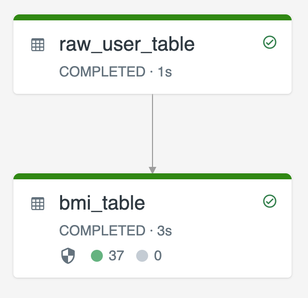
The following diagram illustrates an example using two streaming tables:
raw_user_tableingests raw user data from a source.bmi_tableincrementally computes BMI scores using weight and height fromraw_user_table.
You want to manually delete or update user records from the raw_user_table and recompute the bmi_table.
The following code demonstrates setting the pipelines.reset.allowed table property to false to disable full refresh for raw_user_table so that intended changes are retained over time, but downstream tables are recomputed when a pipeline update is run:
CREATE OR REFRESH STREAMING TABLE raw_user_table
TBLPROPERTIES(pipelines.reset.allowed = false)
AS SELECT * FROM STREAM read_files("/databricks-datasets/iot-stream/data-user", format => "csv");

CREATE OR REFRESH STREAMING TABLE bmi_table
AS SELECT userid, (weight/2.2) / pow(height*0.0254,2) AS bmi FROM STREAM(raw_user_table);