Batch vs. streaming data processing in Databricks

This article describes the key differences between batch and streaming, two different data processing semantics used for data engineering workloads, including ingestion, transformation, and real-time processing.

Streaming is commonly associated with low-latency and continuous processing from message buses, such as Apache Kafka.

However, in Databricks it has a more expansive definition. The underlying engine of DLT (Apache Spark and Structured Streaming) has a unified architecture for batch and streaming processing:

• The engine can treat sources like cloud object storage and Delta Lake as streaming sources for efficient incremental processing.
• Streaming processing can be run in both triggered and continuous manners, giving you the flexibility to control cost and performance tradeoffs for your streaming workloads.

Below are the fundamental semantic differences that distinguish batch and streaming, including their advantages and disadvantages, and considerations for choosing them for your workloads.

Batch semantics

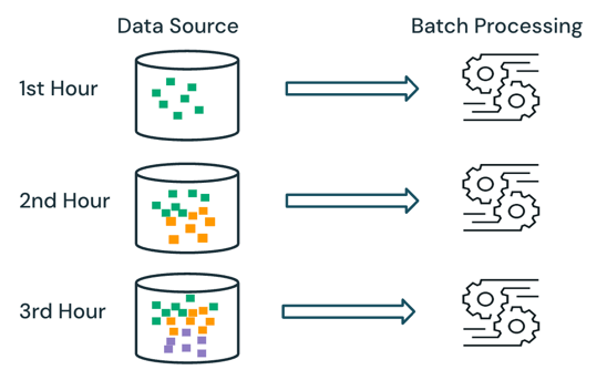
With batch processing, the engine does not keep track of what data is already being processed in the source. All of the data currently available in the source is processed at the time of processing. In practice, a batch data source is typically partitioned logically, for example, by day or region, to limit data reprocessing.

For example, calculating the average item sales price, aggregated at an hourly granularity, for a sales event run by an e-commerce company can be scheduled as batch processing to calculate the average sales price every hour. With batch, data from previous hours is reprocessed each hour, and the previously calculated results are overwritten to reflect the latest results.

Streaming semantics

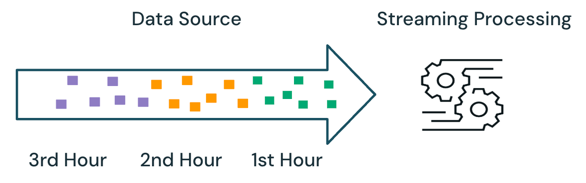
With streaming processing, the engine keeps track of what data is being processed and only processes new data in subsequent runs. In the example above, you can schedule streaming processing instead of batch processing to calculate the average sales price every hour. With streaming, only new data added to the source since the last run is processed. The newly calculated results must be appended to the previously calculated results to check the complete results.

Batch vs. streaming

In the example above, streaming is better than batch processing because it does not process the same data processed in previous runs. However, streaming processing gets more complex with scenarios like out-of-order and late arrival data in the source.

An example of late arrival data is if some sales data from the first hour does not arrive at the source until the second hour:

• In batch processing, the late arrival data from the first hour will be processed with data from the second hour and existing data from the first hour. The previous results from the first hour will be overwritten and corrected with the late arrival data.
• In streaming processing, the late-arriving data from the first hour will be processed without any of the other first-hour data that has been processed. The processing logic must store the sum and count information from the first hour's average calculations to correctly update the previous results.

These streaming complexities are typically introduced when the processing is stateful, such as joins, aggregations, and deduplications.

For stateless streaming processing, such as appending new data from the source, handling out-of-order and late arrival data is less complex, as the late arriving data can be appended to the previous results as the data arrives in the source.

The table below outlines the pros and cons of batch and streaming processing and the different product features that support these two processing semantics in Databricks Lakeflow.

	Batch	Streaming
Pros	Processing logic is simple. Results are always accurate and reflect all the available data in the source.	Efficient, only new data is processed. Faster, could handle latency requirements from hours to minutes, seconds, and milliseconds.
Cons	It is not as efficient; data will be reprocessed in a particular batch partition. Slower, could handle latency requirements from hours to minutes, but not seconds or milliseconds.	Processing logic could be complex, especially for stateful processing such as joins, aggregations, deduplications, etc. Results can not always be accurate, considering out-of-order and late arrival data.
Data engineering products	DLT materialized view flow and materialized view. Databricks Runtime - Apache Spark (spark.read.load() and spark.write.save()).	Lakeflow Connect. DLT append flow, apply change flow, streaming table, and sink. Databricks Runtime - Spark Structured Streaming (spark.readStream.load() and spark.writeStream.start()).

Recommendations

The table below outlines the recommended processing semantics based on the characteristics of the data processing workloads at each layer of the medallion architecture.

Medallion layer	Workload characteristics	Recommendation
Bronze	Ingestion workloads. Typically involves no or stateless processing for incremental append from data sources. The size of data is typically larger.	Streaming processing is generally a better choice, given users can benefit from the advantages of streaming but not get exposed to the complexities of stateful streaming processing.
Silver	Transformation workloads. Typically involves both stateless processing such as filtering and stateful processing such as joins, aggregations, and deduplications.	Use batch processing (with incremental refresh in materialized views) to avoid the complexities of stateful streaming processing. Use streaming processing as an option for use cases where efficiency and latency is much more important than results accuracy. Be mindful of the complexities introduced by stateful streaming processing.
Gold	Last-mile aggregation workloads. Typically involves stateful processing such as joins and aggregations. The size of data is generally smaller.	Use batch processing (with incremental refresh in materialized views) to avoid the complexities of stateful streaming processing.